18 TRR/FER subclone analysis

This section produces all the figures used for Figure 4.

# Source setup file
source("./functions/setup.R")

# Load functions
source("./functions/plotHeatmap.R")

18.1 Plotting deleted genes from TRR/FER subclones

profiles = fread("./data/subclones/P3_median_cn.tsv")
clones = fread("./data/subclones/P3_clones.tsv")
cosmic = fread("./data/genelists/cosmic_gene-census.tsv")
annot = fread("./annotation/P3.tsv", header = F)

# Merge clones with annot
clones[, library := gsub("_.*", "", sample_id)]
clones_annot = merge(clones, annot, by.x = "library", by.y = "V1")

# Select clones that are only present in cancer/focal
total = clones_annot[, .(paste(unique(V3), collapse = ";")), by = cluster]
clones_selected = total[!grepl("Normal", V1)]

# Get selected
profiles = profiles[cluster %in% clones_selected$cluster]
profiles = profiles[(total_cn != 2 & chr != "X") | (total_cn != 1 & chr == "X")]

# Get overlaps
setkey(profiles, chr, start, end)
setkey(cosmic, chr, start, end)
overlaps = foverlaps(cosmic, profiles)[!is.na(total_cn)]
overlaps[, alteration := ifelse(total_cn < 2, "Deleted", "Amplified")]

# Get unique
unique_overlaps = unique(overlaps[, .(name, gene, alteration)])

# Make oncoprint
unique_overlaps_wide = dcast(unique_overlaps, name ~ gene, value.var = "alteration")
mat = as.matrix(unique_overlaps_wide[, 2:ncol(unique_overlaps_wide)])
rownames(mat) = unique_overlaps_wide$name

# Plot oncoprint
# colors
cols = brewer.pal(3, "Set1")[c(1, 2)]
names(cols) = c("Amplified", "Deleted")

oncoPrint(t(mat),
          alter_fun = list(
            background = alter_graphic("rect", width = 0.9, height = 0.9, fill = "#FFFFFF", col = "black", size = .1),
            Amplified = alter_graphic("rect", width = 0.85, height = 0.85, fill = cols["Amplified"]),
            Deleted = alter_graphic("rect", width = 0.85, height = 0.85, fill = cols["Deleted"])),
          col = cols, border = "black", show_column_names = T, show_row_names = T, remove_empty_rows = T,
          show_pct = F, row_names_gp = gpar(fontsize = 17), column_names_gp = gpar(fontsize = 22))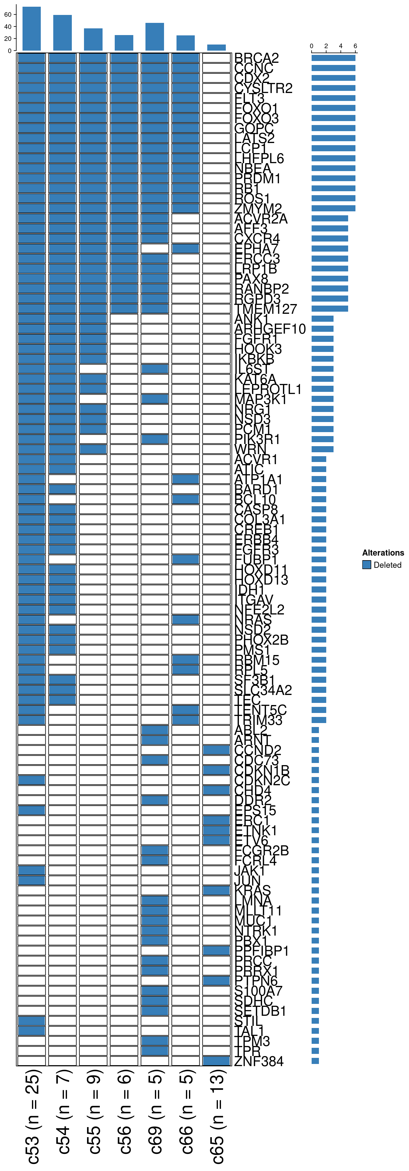

Distributions of the cells belonging to these subclones can be found in the Supplementary Figure 12-15 section.

18.2 Co-deletions of TSGs

To see where the cells harbouring deletions of multiple genes simultaneously are located, we go back to single-cell level (from subclonal level) and plot these cells in the prostate heatmaps.

# Load in data
count_all = readRDS("./data/P3_cnv.rds")$stats
profiles = readRDS("./data/P3_pseudodiploid_500kb.rds")
cosmic = fread("./data/genelists/cosmic_gene-census.tsv")
annot = fread("./annotation/P3.tsv", header = F)
clones = fread("./data/subclones/P3_clones.tsv")

# Get cosmic genes that are amp/del
dt = pivot_longer(profiles, cols = colnames(profiles[, 4:ncol(profiles)]))
setDT(dt)
dt = dt[value != 2, ]
dt[, value := ifelse(value < 2, "Deleted", "Amplified")]

# Setkeys
setkey(dt, chr, start, end)
setkey(cosmic, chr, start, end)

# Get overlap with COSMIC
overlap = foverlaps(cosmic, dt)
overlap = overlap[complete.cases(overlap)]
overlap = unique(overlap, by = c("name", "value", "gene"))

# Merge overlap with section info and subclone info
overlap[, library := gsub("_.*", "", name)]
dt = merge(overlap, annot, by.x = "library", by.y = "V1")
#dt = merge(dt, clones, by.x = "name", by.y = "sample_id")

# Subclones and genes to check
genes_check = c("FOXO1", "FOXO3", "RB1", "BRCA2", "CCNC", "CDX2", "LATS2", "PRDM1")

# Subset
dt = dt[gene %in% genes_check, ]

# Check co-deletions
codels = dt[, paste(gene, collapse = ";"), by = .(name, V2, value)]
codels_counts = codels[, .N, by = .(V2, V1)]

# Get total number of pseudodiploid per section
total_pseudo = data.table(library = gsub("_.*", "", colnames(profiles[, 4:ncol(profiles)])))
total_pseudo = merge(total_pseudo, annot, by.x = "library", by.y = "V1")
counts_pseudo = total_pseudo[, .(total_pseudo = .N), by = V2]

# Get total cells
count_all[, library := gsub("_.*", "", sample)]
count_all = merge(count_all, annot, by.x = "library", by.y = "V1")
counts_total = count_all[classifier_prediction == "good", .(total = .N), by = .(V2)]

# Get fraction pseudo
codels_counts = merge(codels_counts, counts_pseudo, by = "V2")
codels_counts[, fraction_pseudo := N / total_pseudo]

# Add fraction total
codels_counts = merge(codels_counts, counts_total, by = "V2")
codels_counts[, fraction_total := N / total]

# Plot the combination with all deletions
combination = "LATS2;CDX2;BRCA2;FOXO1;RB1;CCNC;PRDM1;FOXO3"

# Select the combination of interest
dt = codels_counts[V1 == combination]

# Fill all with NAs
fill_dt = data.table(V2 = annot[!V2 %in% dt$V2, V2],
                     V1 = NA,
                     N = NA,
                     total_pseudo = NA,
                     fraction_pseudo = NA,
                     total = NA,
                     fraction_total = NA)
dt = rbindlist(list(dt, fill_dt), use.names = TRUE)

# Add coordinates
dt[, x := as.numeric(gsub("L|C.", "", V2))]
dt[, y := as.numeric(gsub("L.|C", "", V2))]

# Plot the number of cells with co-deletion
ggplot(dt, aes(x = x, y = y, fill = N, label = N)) +
  geom_tile() +
  geom_text(size = 7) +
  labs(title = paste0(combination, " deletions")) +
  scale_fill_distiller(name = "Cells with deletion", palette = "Reds", direction = 1, na.value = "grey") +
  geom_hline(yintercept = seq(from = .5, to = max(dt$y), by = 1)) +
  geom_vline(xintercept = seq(from = .5, to = max(dt$x), by = 1)) +
  scale_y_reverse(expand = c(0, 0), breaks = seq(1, max(dt$y)), labels = seq(1, max(dt$y))) + 
  scale_x_reverse(expand = c(0, 0), breaks = seq(1, max(dt$x)), labels = seq(1, max(dt$x))) +
  theme(axis.title = element_blank())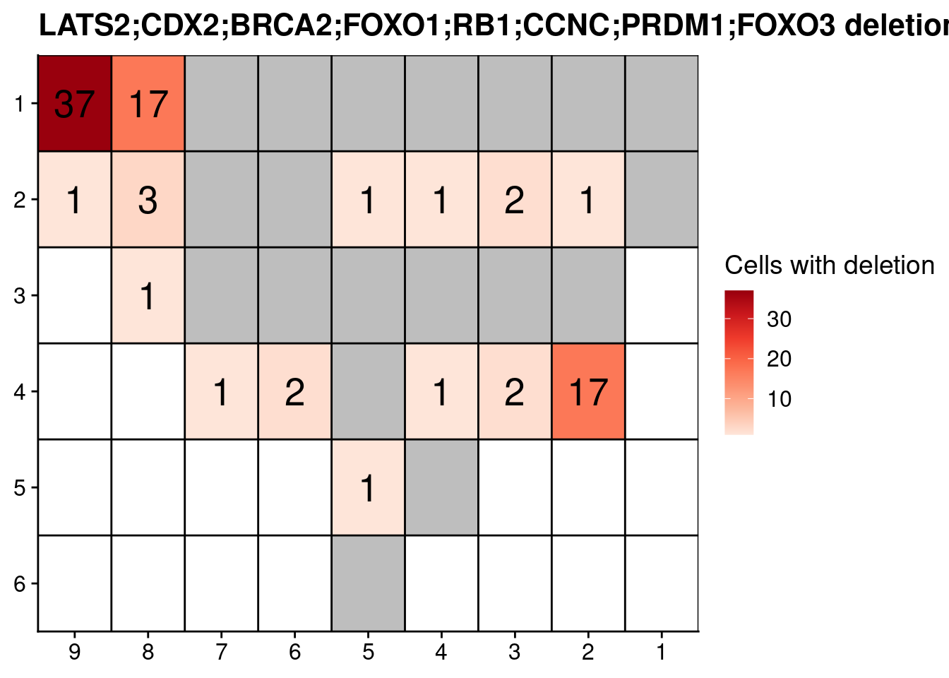

# Plot fraction of pseudodiploid cells
ggplot(dt, aes(x = x, y = y, fill = fraction_pseudo, label = N)) +
  geom_tile() +
  geom_text(size = 7) +
  labs(title = paste0(combination, " deletions")) +
  scale_fill_distiller(name = "fraction of all\npseudo-diploid cells", palette = "Reds", direction = 1, na.value = "grey", labels = scales::percent_format(), limits = c(0, 1)) +
  geom_hline(yintercept = seq(from = .5, to = max(dt$y), by = 1)) +
  geom_vline(xintercept = seq(from = .5, to = max(dt$x), by = 1)) +
  scale_y_reverse(expand = c(0, 0), breaks = seq(1, max(dt$y)), labels = seq(1, max(dt$y))) + 
  scale_x_reverse(expand = c(0, 0), breaks = seq(1, max(dt$x)), labels = seq(1, max(dt$x))) +
  theme(axis.title = element_blank())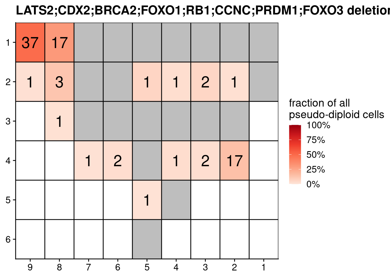

# Plot fraction of total cells
ggplot(dt, aes(x = x, y = y, fill = fraction_total, label = N)) +
  geom_tile() +
  geom_text(size = 7) +
  labs(title = paste0(combination, " deletions")) +
  scale_fill_distiller(name = "fraction of\nall cells", palette = "Reds", direction = 1, na.value = "grey", labels = scales::percent_format(), limits = c(0, 1)) +
  geom_hline(yintercept = seq(from = .5, to = max(dt$y), by = 1)) +
  geom_vline(xintercept = seq(from = .5, to = max(dt$x), by = 1)) +
  scale_y_reverse(expand = c(0, 0), breaks = seq(1, max(dt$y)), labels = seq(1, max(dt$y))) + 
  scale_x_reverse(expand = c(0, 0), breaks = seq(1, max(dt$x)), labels = seq(1, max(dt$x))) +
  theme(axis.title = element_blank())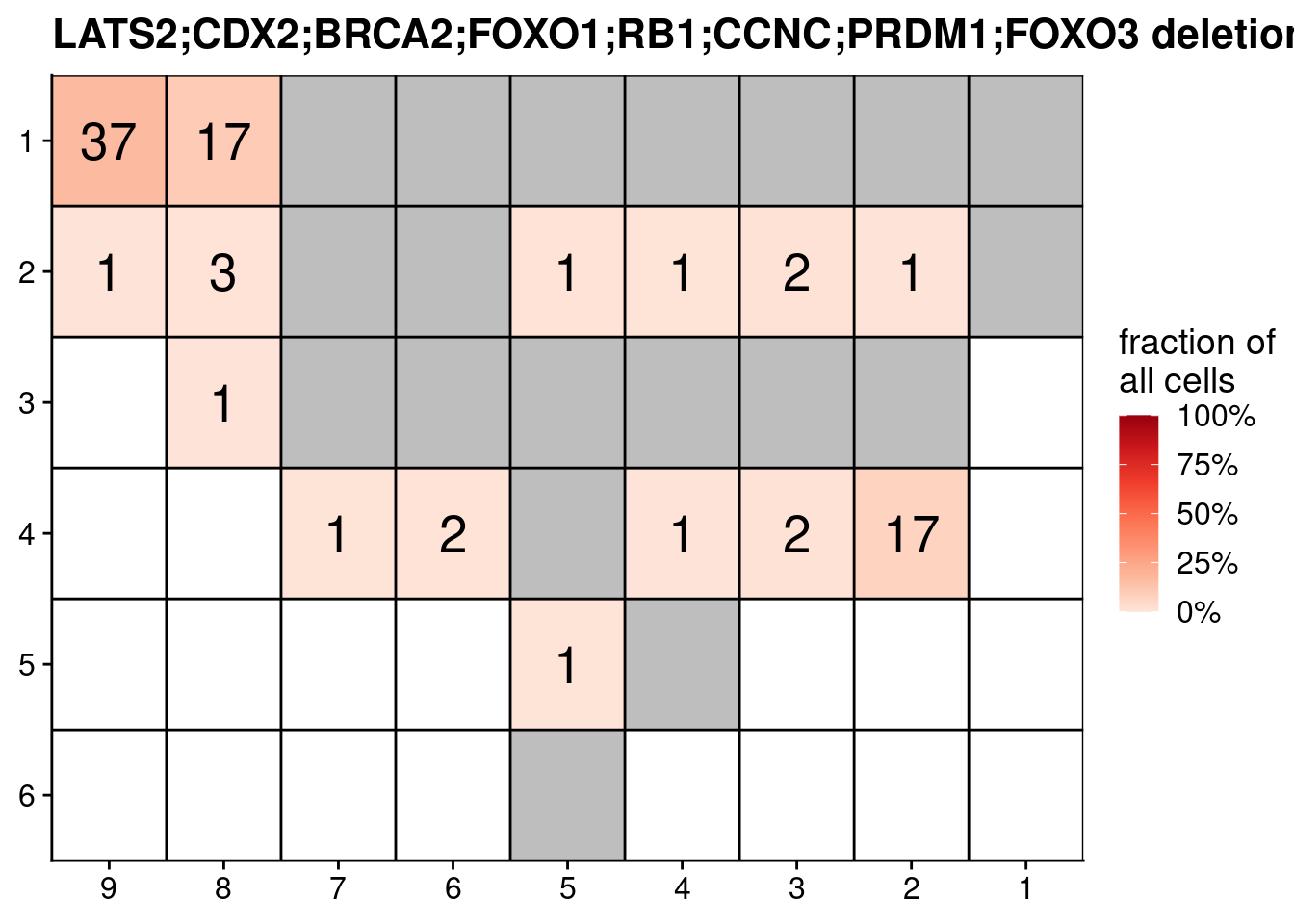

18.3 TCGA deletion analysis

Next, we wanted to see if these deletions are also present (and enriched) in the Prostate Adenocarcinoma (PRAD) TCGA dataset. First we looked into enrichment of deletions of certain genomic regions in TCGA. We used GISTIC2 for this. You can download the TCGA copy number data at cbioportal. Then we ran GISTIC2 with the following command:

gistic2 gp_gistic2_from_seg -b {base_dir} -gcm extreme -seg {TCGA_copynumber_segment_file} -maxseg 2000 -broad 1 -ta 0.1 -td 0.1 -conf 0.99 -brlen 0.7 -armpeel 1

We then used the scores.gistic output file from GISTIC2 to visualize the signficantly deleted (and amplified) regions in PRAD.

# Load GISTIC data
dt = fread("./data/TCGA/scores.gistic")

# Make wide
dt_amp = dt[Type == "Amp", .(chr = paste0("chr", Chromosome), start = Start, end = End, qvalue = -1*`-log10(q-value)`)]
dt_del = dt[Type == "Del", .(chr = paste0("chr", Chromosome), start = Start, end = End, qvalue = `-log10(q-value)`)]

circos.clear()
circos.par("start.degree" = 90, "gap.degree" = c(rep(1, 21), 10), points.overflow.warning=FALSE, track.height = 0.25, track.margin = c(0.01, 0))
circos.initializeWithIdeogram(plotType = c("ideogram", "axis", "labels"), chromosome.index = paste0("chr", 1:22))
# Plot deletion q value track
circos.genomicTrack(dt_del, ylim = c(0, 100), panel.fun = function(region, value, ...) {
  circos.genomicLines(region, value, numeric.column = "del", col = "#377EB8", area = TRUE)
})
circos.yaxis(side = "left", at = c(0, 50, 100), labels = c(0, 50, 100), sector.index = "chr1", labels.niceFacing = TRUE)

# Plot amplification q value track
circos.genomicTrack(dt_amp, ylim = c(-10, 0), panel.fun = function(region, value, ...) {
  circos.genomicLines(region, value, numeric.column = "amp", col = "#E41A1C", area = TRUE, baseline = "top", type = "l")
})
circos.yaxis(side = "left", at = c(-10, -5, 0), labels = c(10, 5, 0), sector.index = "chr1", labels.niceFacing = TRUE)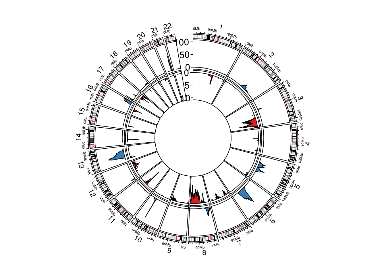

Next, we checked the mutation-status (deletions/amplfications/SNVs) of the genes that we found commonly deleted in our samples in TCGA PRAD. For this we load in the CNA data (.seg file) and we download the mutation data. Note, the downloading and loading of the mutation data can take a couple of minutes.

# Load TCGA data
segments = fread("./data//TCGA/TCGA_firehose-segments.seg")
clinical = fread("./data/TCGA/TCGA_firehose_clinical_data_patient.txt")
cosmic = fread("./data/genelists/cosmic_gene-census.tsv")

# Download mutation data
res = GDCquery(project = "TCGA-PRAD", data.category = "Simple Nucleotide Variation", access = "open",
               data.type = "Masked Somatic Mutation", workflow.type = "Aliquot Ensemble Somatic Variant Merging and Masking")
GDCdownload(res, directory = "./data/TCGA/gdc_query/")
tcga_muts = GDCprepare(res, directory = "./data/TCGA/gdc_query/")

# Set as data.table and rename columns for ease of use
setDT(tcga_muts)
setnames(tcga_muts, "Gene", "gene")

# Get actual patient ID
tcga_muts[, ID := gsub("-0.*|-0.*", "", Tumor_Sample_Barcode)]
segments[, ID := gsub("-0.*", "", ID)]

# Select IDs that are in cn data and vice versa
tcga_muts = tcga_muts[ID %in% segments$ID & Variant_Classification == "Missense_Mutation", .(ID, Hugo_Symbol)]
tcga_muts[, alteration := "SNV"]
setnames(tcga_muts, "Hugo_Symbol", "gene")

# Select only IDs that are also in the mutation data.table
segments = segments[ID %in% tcga_muts$ID]

# Setnames
setnames(segments, c("ID", "chr", "start", "end", "num_mark", "segmean"))

# Get deletions only and remove X from cosmic
segments[segmean <= -.5, alteration := "Deleted"]
segments[segmean >= .5, alteration := "Amplified"]
segments = segments[!is.na(alteration), ]

cosmic = cosmic[chr != "X",]
cosmic[, chr := as.integer(chr)]

# Setkeys
setkey(segments, chr, start, end)
setkey(cosmic, chr, start, end)

# Get overlap with COSMIC
overlap = foverlaps(cosmic, segments)
overlap = overlap[complete.cases(overlap)]

# Get unique IDS
overlap = unique(overlap, by = c("ID", "gene"))

# Merge with mutations
overlap = overlap[, .(ID, alteration, gene)]
overlap = rbind(overlap, tcga_muts[, .(ID, gene, alteration)])

# Select genes
genes_select = c("FOXO1", "FOXO3", "FOXP1", "RB1", "CCNC", "CDX2", "LATS2", "PRDM1", "BRCA2")
overlap = overlap[gene %in% genes_select, ]

# Dcast 
result = dcast(overlap, gene ~ ID, value.var = "alteration", fun.aggregate = function(x) paste(x, collapse = ";"))

# Prepare oncoprint
cols = brewer.pal(3, "Set1")[c(1, 2, 3)]
names(cols) = c("Amplified", "Deleted", "SNV")

mat = as.matrix(result[, 2:ncol(result)])
rownames(mat) = result[[1]]

# Add clinical Gleason score
clinical = clinical[, .(PATIENT_ID, GLEASON_SCORE, GLEASON_PATTERN_PRIMARY, GLEASON_PATTERN_SECONDARY)]
clinical[, gleason := paste0(GLEASON_PATTERN_PRIMARY, "+", GLEASON_PATTERN_SECONDARY)]

# Assign clinical grade groups based on gleason
clinical[GLEASON_SCORE == 6, grade_group := "Grade Group 1"]
clinical[gleason == "3+4", grade_group := "Grade Group 2"]
clinical[gleason == "4+3", grade_group := "Grade Group 3"]
clinical[GLEASON_SCORE == 8, grade_group := "Grade Group 4"]
clinical[GLEASON_SCORE > 8, grade_group := "Grade Group 5"]

# Add annotation and reorder
clinical = clinical[PATIENT_ID %in% colnames(mat), ]
clinical = clinical[match(colnames(mat), PATIENT_ID)]

#annot_cols = list("Gleason score" = c("Gleason low" = brewer.pal(3, "Set1")[2], "Gleason high" = brewer.pal(3, "Set1")[1]))
annot_cols = list("Grade Group" = c("Grade Group 1" = pal_npg()(5)[1], "Grade Group 2" = pal_npg()(5)[2], "Grade Group 3" = pal_npg()(5)[3],
                                    "Grade Group 4" = pal_npg()(5)[4], "Grade Group 5" = pal_npg()(5)[5]))
onco_annot = HeatmapAnnotation(`Grade Group` = clinical$grade_group, col = annot_cols)

#plot
oncoPrint(mat,
          alter_fun = list(
            background = alter_graphic("rect", width = 0.9, height = 0.9, fill = "#FFFFFF", col = "black", size = .1),
            Amplified = alter_graphic("rect", width = 0.85, height = 0.9, fill = cols["Amplified"]),
            Deleted = alter_graphic("rect", width = 0.85, height = 0.9, fill = cols["Deleted"]),
            SNV = alter_graphic("rect", width = 0.85, height = 0.45, fill = cols["SNV"])), 
          col = cols, border = "black", show_column_names = F, show_row_names = T, remove_empty_rows = T,
          show_pct = F, row_names_gp = gpar(fontsize = 10), top_annotation = NULL, bottom_annotation = onco_annot)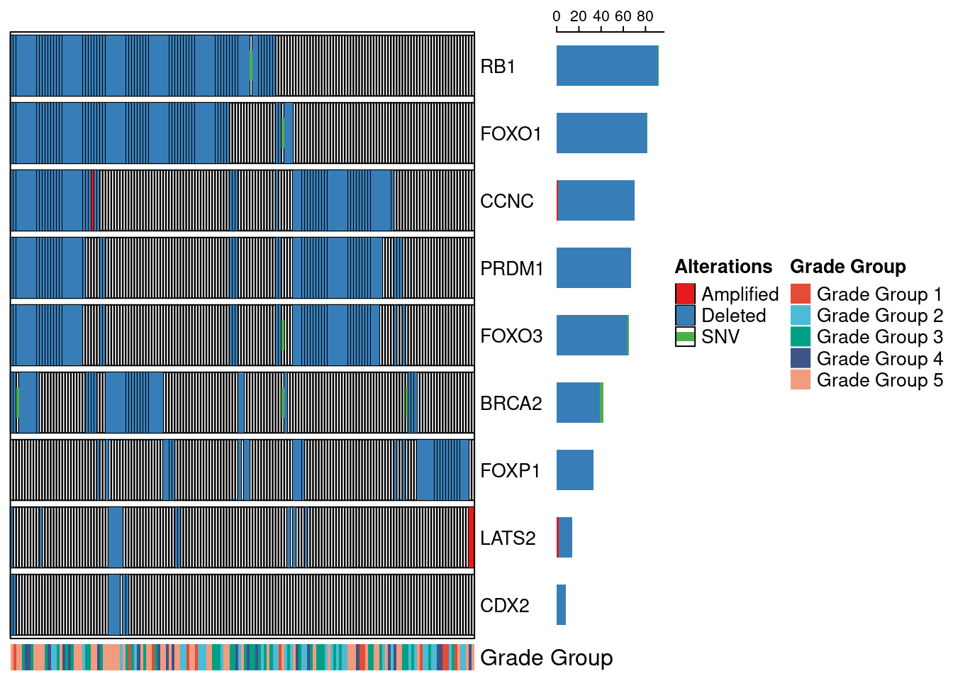

18.4 Targeted sequencing mutations

Finally, we also plot the mutation data of certain genes from our targeted deep sequencing.

muts = fread("./data/mutations/P3_filtered_SNVs.tsv")
annot = fread("./annotation/P3.tsv", header = FALSE, col.names = c("library", "section", "pathology"))

# Remove underscore in sample
muts[, SAMPLE := gsub("_", "", SAMPLE)]

# Remove LOC/2nd genes
muts[, GeneName := gsub("LOC.*:", "", GeneName)]
muts[, GeneName := gsub(":.*", "", GeneName)]

# Get number of mutations
num_muts = muts[, .N, by = SAMPLE]
num_muts[, SAMPLE := gsub("P.", "", SAMPLE)]
setnames(num_muts, c("section", "n_muts"))

# Merge with annotation
num_muts = merge(num_muts, annot, by = "section")

# Add coordinates
num_muts[, x := as.numeric(gsub("L|C.", "", section))]
num_muts[, y := as.numeric(gsub("L.|C", "", section))]

# Fill dt
fill_dt = data.table(section = annot[!section %in% num_muts$section, section],
                     n_muts = NA,
                     library = NA,
                     pathology = NA)
fill_dt[, x := as.numeric(gsub("L|C.", "", section))]
fill_dt[, y := as.numeric(gsub("L.|C", "", section))]
num_muts = rbind(num_muts, fill_dt)

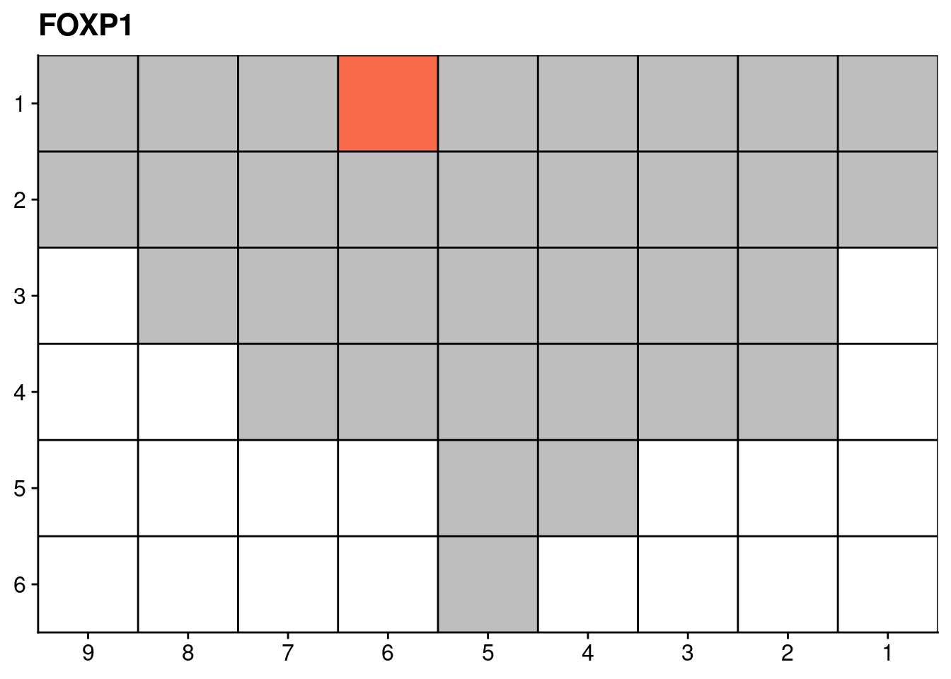
# Plot gene specific heatmaps
genelist = c("LRP1B", "SPTA1", "SPOP", "FOXA1", "FOXP1")

lapply(genelist, function(gene) {
  dt = muts[GeneName == gene, .(count = .N), by = .(SAMPLE)]
  
  # Add sections
  dt = rbind(dt, num_muts[, .(SAMPLE = section, count = NA)])
  dt = dt[, .(count = sum(count, na.rm = T)), by = SAMPLE]
  dt[count == 0, count := NA]
  
  # Add coordinates
  dt[, x := as.numeric(gsub("L|C.", "", SAMPLE))]
  dt[, y := as.numeric(gsub("L.|C", "", SAMPLE))]
  
  # Plot
  ggplot(dt, aes(x = x, y = y, fill = count)) +
    geom_tile() +
    labs(title = gene) +
    scale_fill_distiller(name = "Number of somatic\nnon-synonymous\nmutations detected", palette = "Reds", direction = 1, na.value = "grey") +
    geom_hline(yintercept = seq(from = .5, to = max(dt$y), by = 1)) +
    geom_vline(xintercept = seq(from = .5, to = max(dt$x), by = 1)) +
    scale_y_reverse(expand = c(0, 0), breaks = seq(1, max(dt$y)), labels = seq(1, max(dt$y))) + 
    scale_x_reverse(expand = c(0, 0), breaks = seq(1, max(dt$x)), labels = seq(1, max(dt$x))) +
    theme(axis.title = element_blank(),
          legend.position = "none")
})

## [[1]]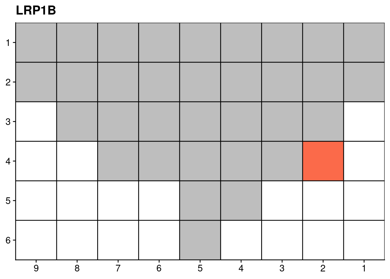

## 
## [[2]]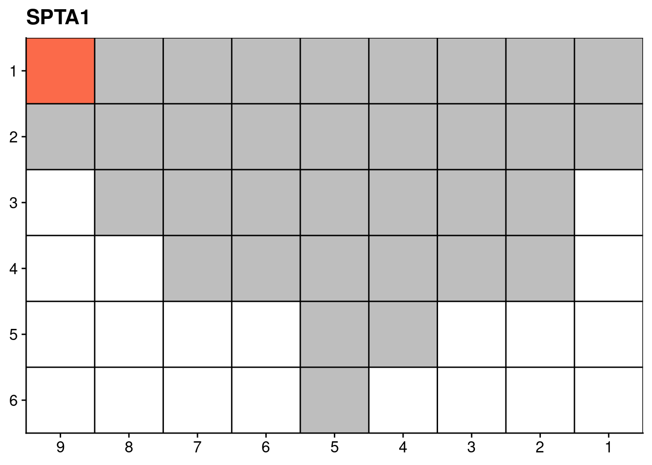

## 
## [[3]]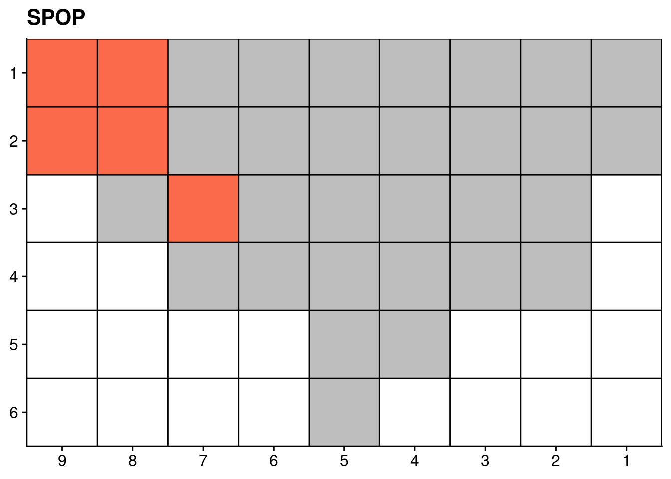

## 
## [[4]]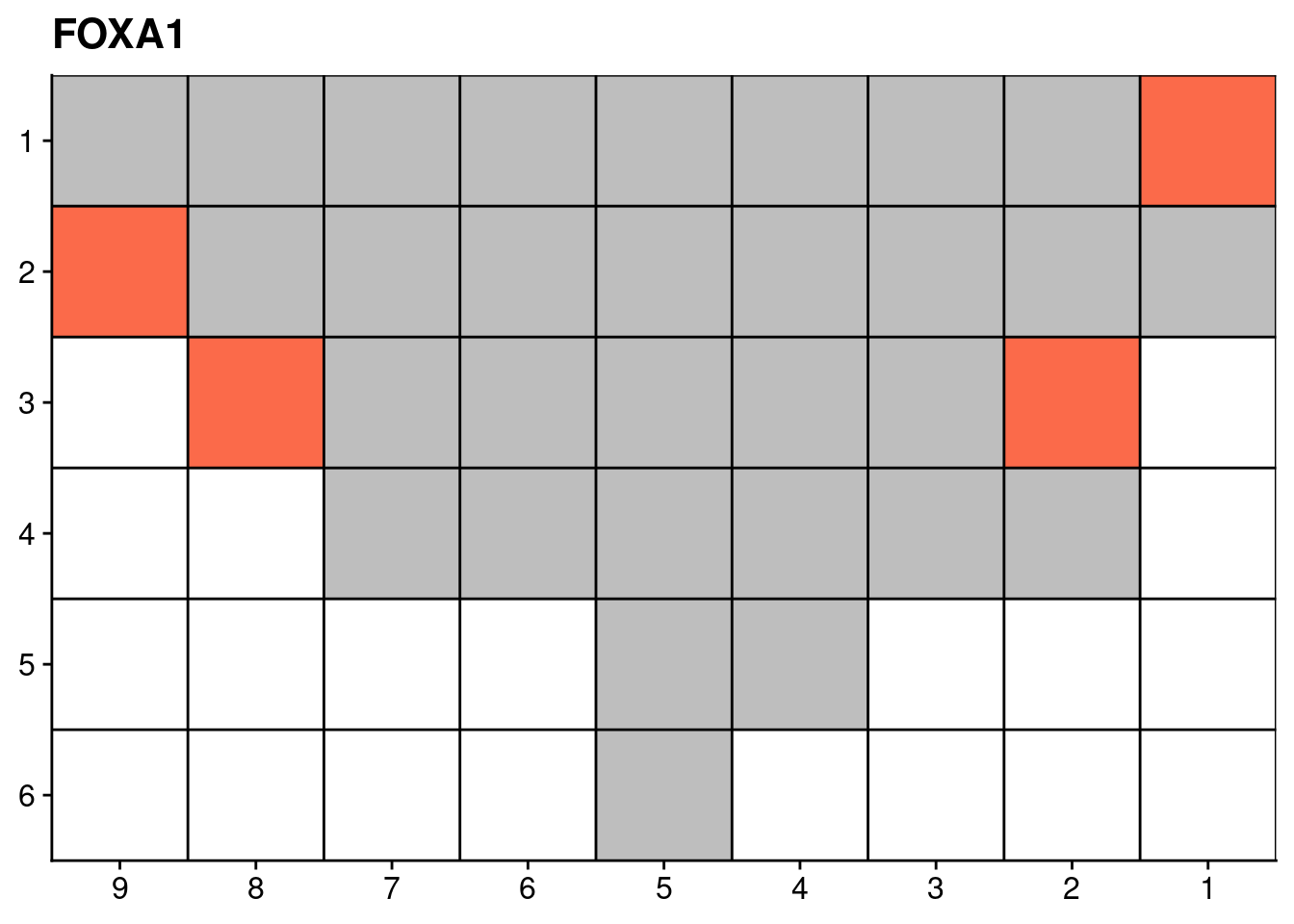

## 
## [[5]]