9 Copy number profiles of other prostate cancer patients
This sections produces all the figures used in Supplementary Figure 7.
# Source setup file
source("./functions/setup.R")

# Load functions
source("./functions/plotHeatmap.R")
9.1 Plot genomewide heatmap
First we look at the overall copynumber profiles of the other 4 prostate cancer patients. We sequenced 2 sections (96 cells input) for each patient.
# Load data
P2 = readRDS("./data/P2_cnv.rds")
P4 = readRDS("./data/P4_cnv.rds")
P5 = readRDS("./data/P5_cnv.rds")
P7 = readRDS("./data/P7_cnv.rds")

# Select HQ cells
p2_profiles = P2$copynumber[, P2$stats[classifier_prediction == "good", sample], with = FALSE]
p4_profiles = P4$copynumber[, P4$stats[classifier_prediction == "good", sample], with = FALSE]
p5_profiles = P5$copynumber[, P5$stats[classifier_prediction == "good", sample], with = FALSE]
p7_profiles = P7$copynumber[, P7$stats[classifier_prediction == "good", sample], with = FALSE]

# Set blocks to block 1 and 2
setnames(p2_profiles, gsub("L6C3", "P2_block1", colnames(p2_profiles)))
setnames(p2_profiles, gsub("P2L2C3", "P2_block2", colnames(p2_profiles)))

setnames(p4_profiles, gsub("L6C4", "P4_block1", colnames(p4_profiles)))
setnames(p4_profiles, gsub("L2C3", "P4_block2", colnames(p4_profiles)))

setnames(p5_profiles, gsub("L7C5", "P5_block1", colnames(p5_profiles)))
setnames(p5_profiles, gsub("L5C5", "P5_block2", colnames(p5_profiles)))

setnames(p7_profiles, gsub("L7C3", "P7_block1", colnames(p7_profiles)))
setnames(p7_profiles, gsub("L3C3", "P7_block2", colnames(p7_profiles)))

# Combine data
total = do.call(cbind, list(p2_profiles, p4_profiles, p5_profiles, p7_profiles))
bins = P2$bins

# Get annotation
annot = data.table(sample = colnames(total),
                   patient = gsub("_.*", "", colnames(total)),
                   block = gsub("P._|_.*", "", colnames(total)))
annot_m = melt(annot, id.vars = "sample")

# Plot heatmap
plotHeatmap(total, bins, annotation = annot_m, linesize = 1.5, rasterize = TRUE)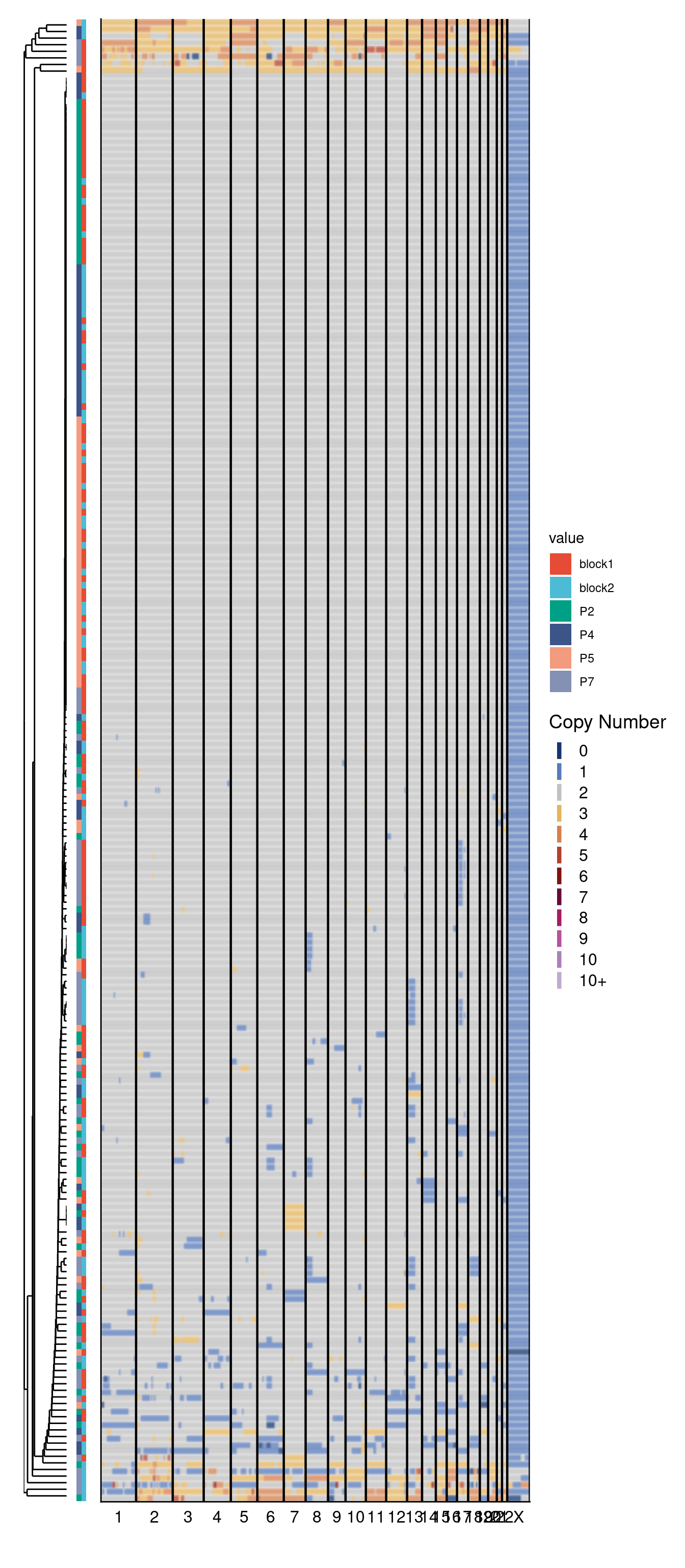
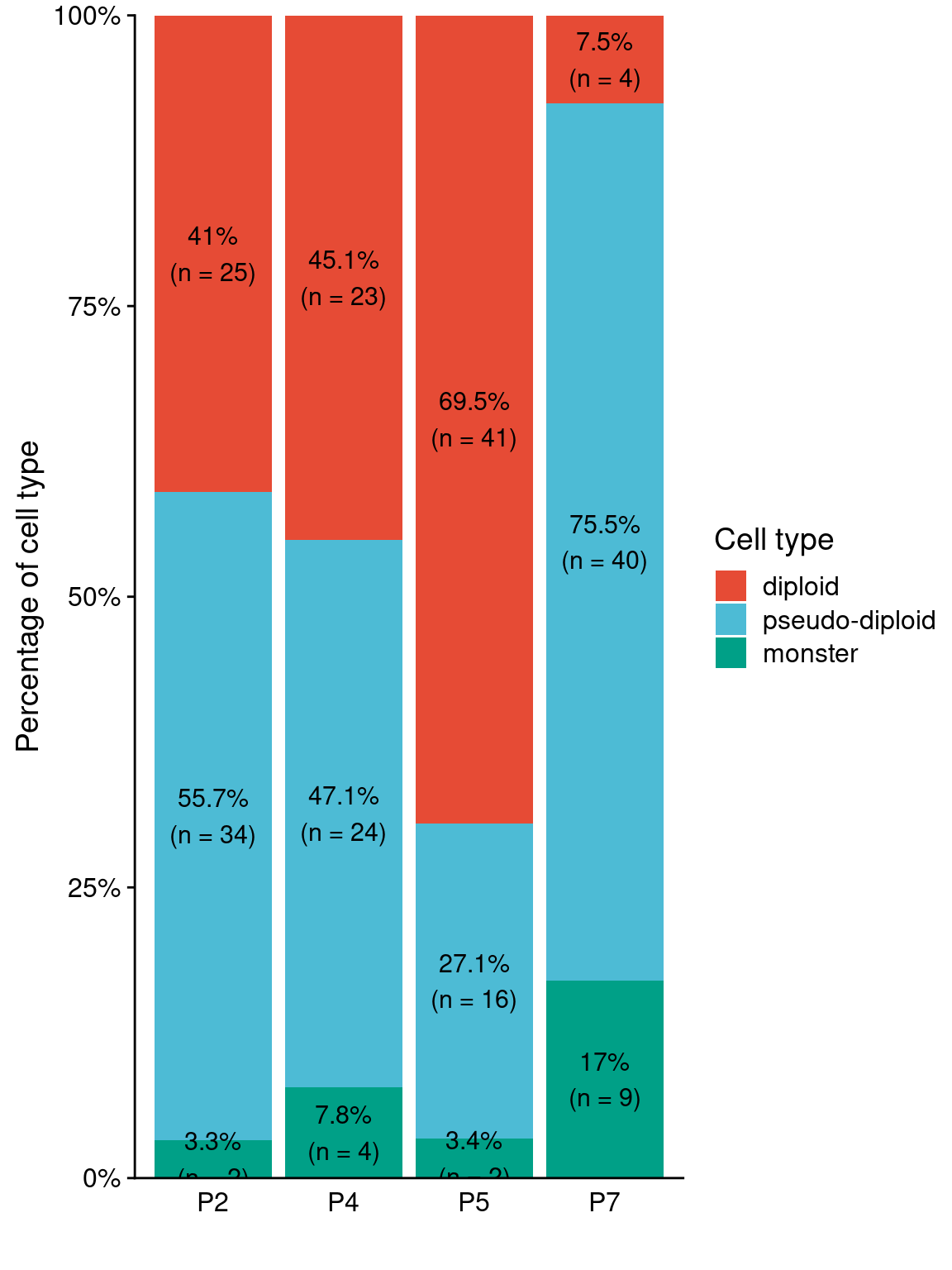
9.2 Plot cell type distribution
Next, we plot the distribution of the three different cell types that we detected earlier in the other 2 prostate cancer samples.
# Set diploid vector to compare against
diploid_vector = c(rep(2, sum(bins$chr != "X")), rep(1, sum(bins$chr == "X")))

# Keep these profiles
diploid_check = sapply(colnames(total), function(cell) {
  sum(total[[cell]] != diploid_vector)
})

dt = data.table(sample = names(diploid_check), num_altered = diploid_check)

# Annotate celltype
dt[num_altered == 0, celltype := "diploid"]
dt[num_altered != 0 & num_altered <= 0.25 * nrow(bins), celltype := "pseudo-diploid"]
dt[num_altered > 0.25 * nrow(bins), celltype := "monster"]

# Get patient info
dt[, patient := gsub("_.*", "", sample)]
counts = dt[, .N, by = .(celltype, patient)]
counts_patient = dt[, .N, by = patient]

# Get fraction
counts = merge(counts, counts_patient, by = "patient")
counts[, fraction := N.x / N.y]

# Set order
counts[, celltype := factor(celltype, levels = c("diploid", "pseudo-diploid", "monster"))]

ggplot(counts, aes(x = patient, y = fraction, fill = celltype, label = N.x)) +
  geom_col() +
  scale_y_continuous(expand = c(0, 0), labels = scales::percent_format()) +
  labs(y = "Percentage of cell type", x = "", fill = "Cell type") +
  geom_text(aes(label = paste0(round(fraction * 100, 1), "%\n(n = ", N.x, ")")),
            position = position_stack(vjust = .5), size = 4) +
  scale_fill_npg() +
  theme(axis.ticks.x = element_blank())