14 Subclonal distribution in prostate
This sections produces all the figures used in Supplementary Figure 11.
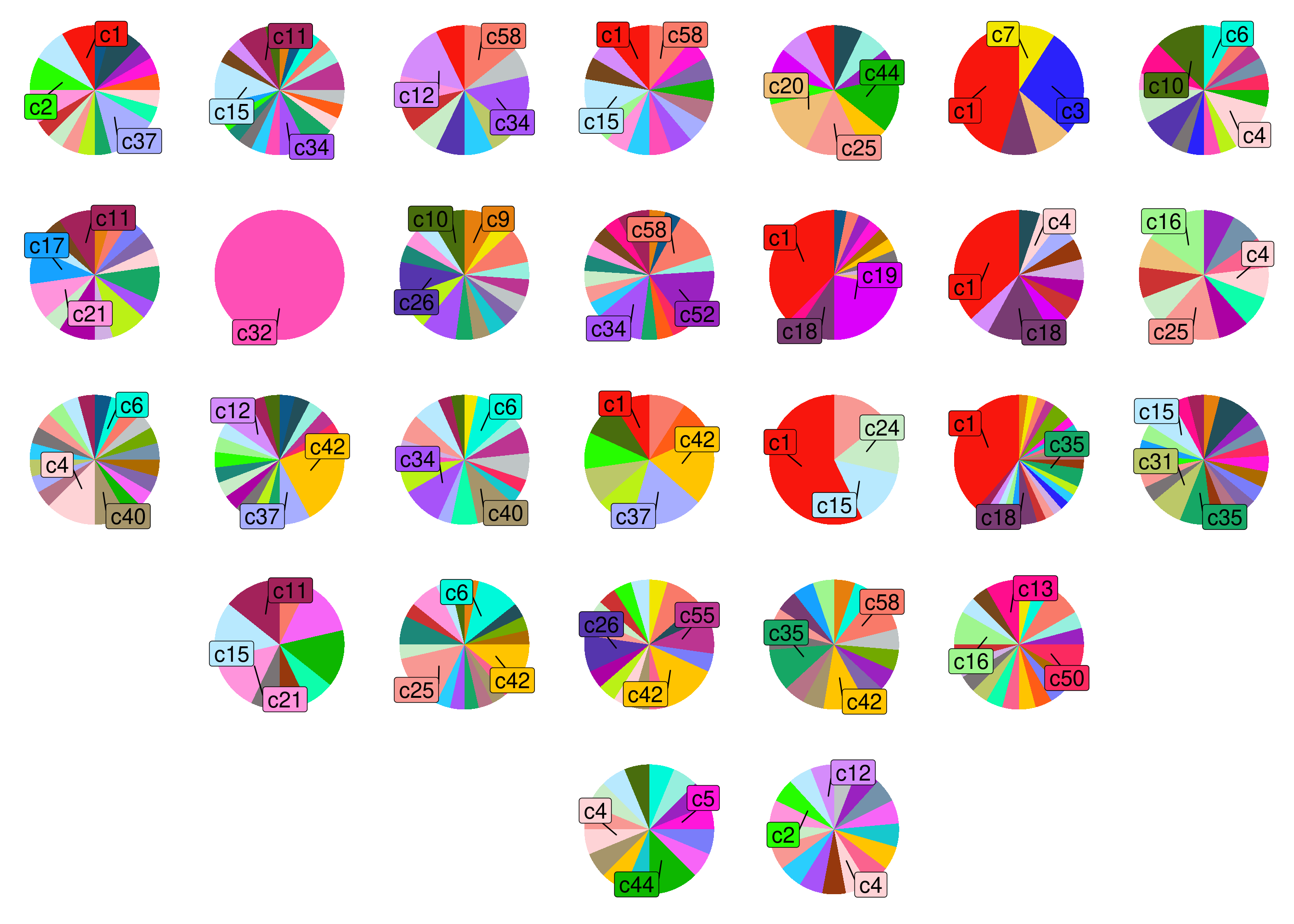
14.1 Plotting spatial subclonal distribution
We plot the spatial subclonal distribution using piecharts and placing them in the spatial location of the section. The code used to generate the file containing the subclone information is included in Figure 2. We also include the final file in this repository.
First we plot P3.
# Load data
clones = fread("./data/subclones/P3_clones.tsv")
annot = fread("./annotation/P3.tsv", header = F)

# Merge clones with annotation data
clones[, library := gsub("_.*", "", sample_id)]
clones = merge(clones, annot, by.x = "library", by.y = "V1")
setnames(clones, "V2", "section")

# Get fraction of each subclone in each section
clones = clones[, .N, by = .(cluster, section)]
clones = clones[, .(cluster = cluster, fraction = N / sum(N)), by = .(section)]

# Add coordinates
clones[, x := as.numeric(gsub("L|C.", "", section))]
clones[, y := as.numeric(gsub("L.|C", "", section))]

# Fill NAs
clones = complete(clones, tidyr::expand(clones, x, y))
setDT(clones)
clones[, section := paste0("L", x, "C", y)]

# Add top 3 indication
setorder(clones, section, -fraction)
clones[, rankings := 1:.N, by = .(section)]
clones[rankings <= 3, label_text := cluster]

# Get label positions
clones =  clones %>%
  group_by(section) %>%
  mutate(text_y = cumsum(fraction) - fraction/2)
setDT(clones)

# Get colors
#colors_vector = get_colors()
col_vector = createPalette(sum(!is.na(unique(clones$cluster))), c("#ff0000", "#00ff00", "#0000ff"))
col_vector = setNames(col_vector, paste0("c", 1:sum(!is.na(unique(clones$cluster)))))

# Set sections
all_sections = unique(clones$section)

# Plot
plots = lapply(all_sections, function(subset) {
  if(is.na(clones[section == subset]$fraction)[1]) {
    plt = ggplot() + theme_void()
  } else {
    plt =
      ggplot(clones[section == subset], aes(x = "", y = fraction, fill = cluster)) +
      geom_col() +
      coord_polar(theta = "y") +
      geom_label_repel(aes(label = label_text),
                       position = position_stack(vjust = .5), size = 6, box.padding = unit(0.6, "lines")) +
      scale_fill_manual(values = col_vector) +
      theme(axis.line = element_blank(),
            axis.text = element_blank(),
            axis.ticks = element_blank(),
            axis.title = element_blank(),
            legend.position = "none")
  }
  return(plt)
})

# Set names
names(plots) = all_sections

# Reorder plots based on tumor location
order = unique(clones, by = "section")
setorder(order, y, -x)
plots = plots[order$section]

# Arrange plots
cowplot::plot_grid(plotlist = plots, nrow = max(order$y), ncol = max(order$x))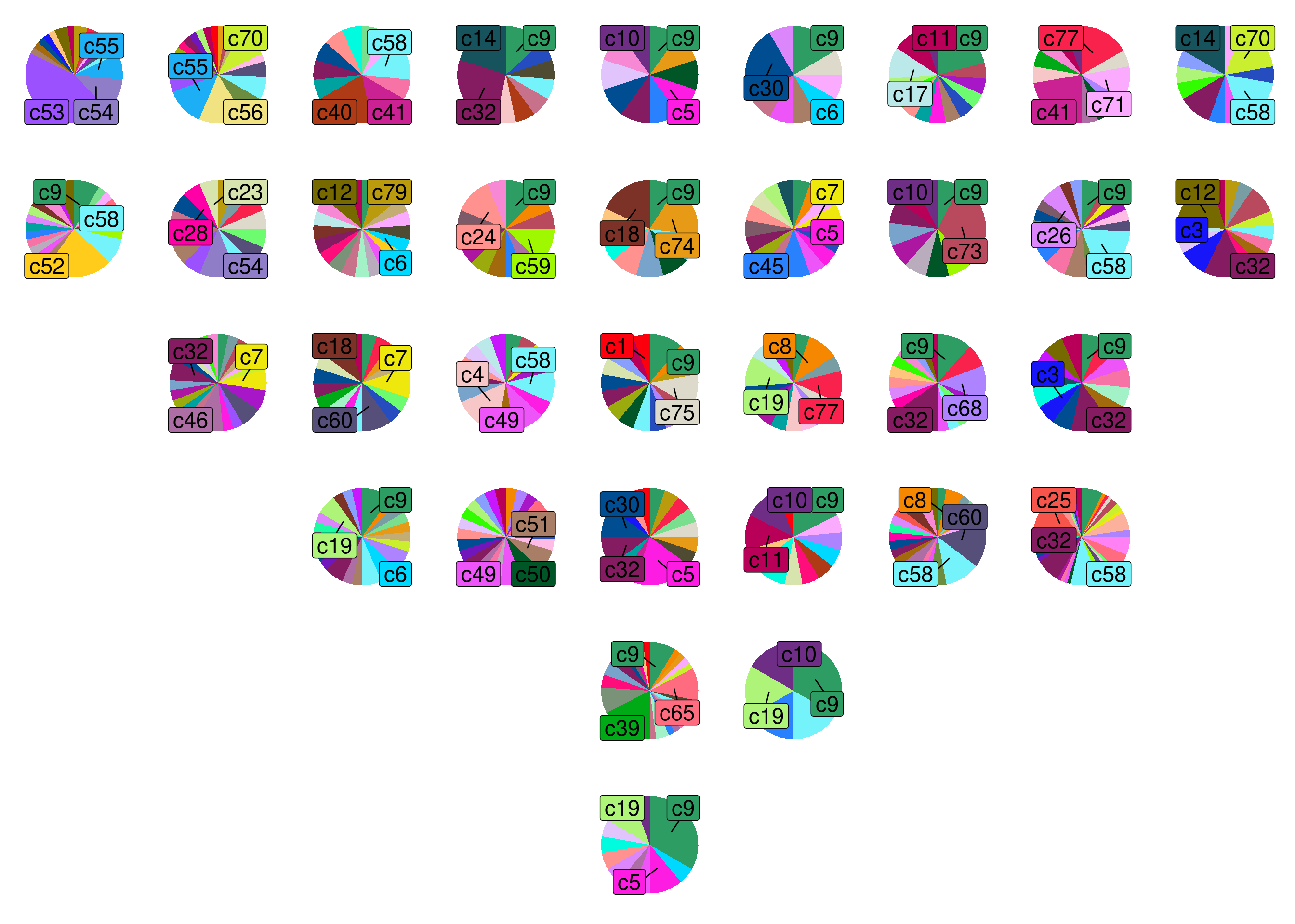
Now we do the same for P6
# Load data
clones = fread("./data/subclones/P6_clones.tsv")
annot = fread("./annotation/P6.tsv", header = F)

# Merge clones with annotation data
clones[, library := gsub("_.*", "", sample_id)]
clones = merge(clones, annot, by.x = "library", by.y = "V1")
setnames(clones, "V2", "section")

# Get fraction of each subclone in each section
clones = clones[, .N, by = .(cluster, section)]
clones = clones[, .(cluster = cluster, fraction = N / sum(N)), by = .(section)]

# Add coordinates
clones[, x := as.numeric(gsub("L|C.", "", section))]
clones[, y := as.numeric(gsub("L.|C", "", section))]

# Fill NAs
clones = complete(clones, tidyr::expand(clones, x, y))
setDT(clones)
clones[, section := paste0("L", x, "C", y)]

# Add top 3 indication
setorder(clones, section, -fraction)
clones[, rankings := 1:.N, by = .(section)]
clones[rankings <= 3, label_text := cluster]

# Get label positions
clones =  clones %>%
  group_by(section) %>%
  mutate(text_y = cumsum(fraction) - fraction/2)
setDT(clones)

# Get colors
#colors_vector = get_colors()
col_vector = createPalette(sum(!is.na(unique(clones$cluster))), c("#ff0000", "#00ff00", "#0000ff"))
col_vector = setNames(col_vector, paste0("c", 1:sum(!is.na(unique(clones$cluster)))))

# Set sections
all_sections = unique(clones$section)

# Plot
plots = lapply(all_sections, function(subset) {
  if(is.na(clones[section == subset]$fraction)[1]) {
    plt = ggplot() + theme_void()
  } else {
    plt =
      ggplot(clones[section == subset], aes(x = "", y = fraction, fill = cluster)) +
      geom_col() +
      coord_polar(theta = "y") +
      geom_label_repel(aes(label = label_text),
                       position = position_stack(vjust = .5), size = 6, box.padding = unit(0.6, "lines")) +
      scale_fill_manual(values = col_vector) +
      theme(axis.line = element_blank(),
            axis.text = element_blank(),
            axis.ticks = element_blank(),
            axis.title = element_blank(),
            legend.position = "none")
  }
  return(plt)
})

# Set names
names(plots) = all_sections

# Reorder plots based on tumor location
order = unique(clones, by = "section")
setorder(order, y, -x)
plots = plots[order$section]

# Arrange plots
cowplot::plot_grid(plotlist = plots, nrow = max(order$y), ncol = max(order$x))