4 Technical validation of scCUTseq
This sections produces all the figures used in Supplementary Figure 1 and 2.
# Source setup file
source("./functions/setup.R")

# Source plotting functions
source("./functions/plotProfile.R")
source("./functions/plotHeatmap.R")
4.1 Duplication rates of CUTseq vs MALBAC
Duplication rate of CUTseq performed on a single cell and MALBAC with different volume scaling.
counts = dup_rate[, .N, by = library]
ggplot(dup_rate, aes(x = library, y = duplication)) +
  geom_violin(aes(fill = library, color = library)) +
  geom_boxplot(width = .075) +
  scale_fill_viridis_d(begin = .3) +
  scale_color_viridis_d(begin = .3) +
  scale_y_continuous(labels = scales::label_percent()) +
  geom_text(data = counts, aes(y = 0.1, x = library, label = paste0("n = ", N))) +
  labs(y = "Duplication rate", x = "") +
  theme(legend.position = "none")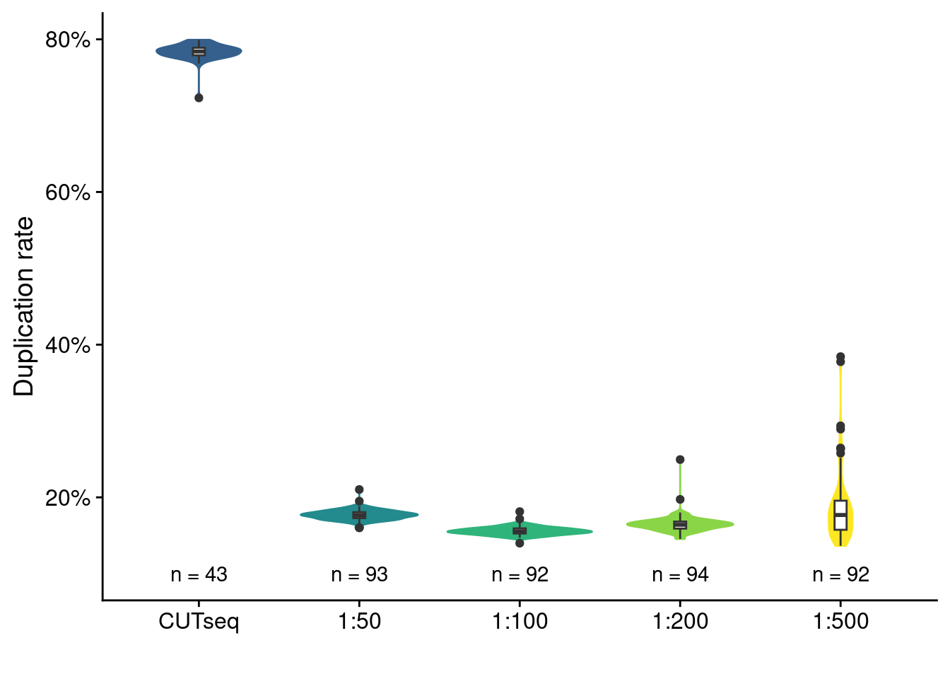
4.2 Pearson correlation MALBAC scaling
Pairwise Pearson correlation between scCUTseq on SKBR3 cells using different MALBAC scalings
ref = readRDS("./data/technical_validation/cnv_SKBR_bulk_CUTseq.rds")
mb50 = readRDS("./data/technical_validation/cnv_MALBAC_50.rds")
mb100 = readRDS("./data/technical_validation/cnv_MALBAC_100.rds")
mb200 = readRDS("./data/technical_validation/cnv_MALBAC_200.rds")
mb500 = readRDS("./data/technical_validation/cnv_MALBAC_500.rds")

# Select copynumbers
ref_cn = ref$copynumber$TGATGCGC
mb50_cn = mb50$copynumber
mb100_cn = mb100$copynumber
mb200_cn = mb200$copynumber
mb500_cn = mb500$copynumber
# Pairwise correlation
mb50_pw = cor(mb50_cn)
mb50_pw = data.table(sample = "1:50",
V1 = rownames(mb50_pw)[row(mb50_pw)[upper.tri(mb50_pw, diag = F)]],
V2 = colnames(mb50_pw)[col(mb50_pw)[upper.tri(mb50_pw, diag = F)]],
pearson = c(mb50_pw[upper.tri(mb50_pw, diag = F)]))
mb100_pw = cor(mb100_cn)
mb100_pw = data.table(sample = "1:100",
V1 = rownames(mb100_pw)[row(mb100_pw)[upper.tri(mb100_pw, diag = F)]],
V2 = colnames(mb100_pw)[col(mb100_pw)[upper.tri(mb100_pw, diag = F)]],
pearson = c(mb100_pw[upper.tri(mb100_pw, diag = F)]))
mb200_pw = cor(mb200_cn)
mb200_pw = data.table(sample = "1:200",
V1 = rownames(mb200_pw)[row(mb200_pw)[upper.tri(mb200_pw, diag = F)]],
V2 = colnames(mb200_pw)[col(mb200_pw)[upper.tri(mb200_pw, diag = F)]],
pearson = c(mb200_pw[upper.tri(mb200_pw, diag = F)]))
mb500_pw = cor(mb500_cn)
mb500_pw = data.table(sample = "1:500",
V1 = rownames(mb500_pw)[row(mb500_pw)[upper.tri(mb500_pw, diag = F)]],
V2 = colnames(mb500_pw)[col(mb500_pw)[upper.tri(mb500_pw, diag = F)]],
pearson = c(mb500_pw[upper.tri(mb500_pw, diag = F)]))
res_pw = rbindlist(list(mb50_pw, mb100_pw, mb200_pw, mb500_pw))
# Prepare for plotting
res_pw[, sample := factor(sample, levels = c("1:50", "1:100", "1:200", "1:500"))]
obs = res_pw[, .N, by = sample]
# Plot
ggplot(res_pw, aes(x = sample, y = pearson)) +
geom_violin(aes(fill = sample)) +
geom_boxplot(width = .04, outlier.size = .5) +
geom_text(data = obs, aes(y = 0, label = paste("n =", N))) +
scale_fill_viridis_d(begin = .4) +
scale_y_continuous(limits = c(0, 1), breaks = seq(0, 1, .2), labels = seq(0, 1, .2)) +
labs(y = "Pairwise Pearson's Correlation", x = "") +
theme(legend.position = "none")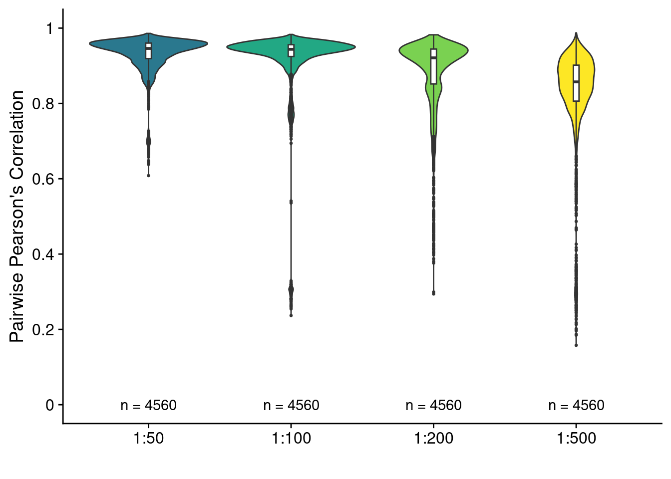
Pearson correlation between scCUTseq with different MALBAC scalings and bulk CUTseq
# Correlation against ref bulk CUTseq
mb50_cor = data.table(sample = "1:50", pearson = as.vector(cor(mb50_cn, ref_cn)))
mb100_cor = data.table(sample = "1:100", pearson = as.vector(cor(mb100_cn, ref_cn)))
mb200_cor = data.table(sample = "1:200", pearson = as.vector(cor(mb200_cn, ref_cn)))
mb500_cor = data.table(sample = "1:500", pearson = as.vector(cor(mb500_cn, ref_cn)))

res = rbindlist(list(mb50_cor, mb100_cor, mb200_cor, mb500_cor))
res[, sample := factor(sample, levels = c("1:50", "1:100", "1:200", "1:500"))]
obs = res[, .N, by = sample]

# Plot
ggplot(res, aes(x = sample, y = pearson)) +
  geom_violin(aes(fill = sample)) +
  geom_boxplot(width = .04, outlier.size = .5) +
  geom_text(data = obs, aes(y = 0, label = paste("n =", N))) +
  scale_fill_viridis_d(begin = .4) +
  scale_y_continuous(limit = c(0, 1), breaks = seq(0, 1, .2), labels = seq(0, 1, .2)) +
  labs(y = "Pearson's Correlation to bulk CUTseq", x = "") +
  theme(legend.position = "none")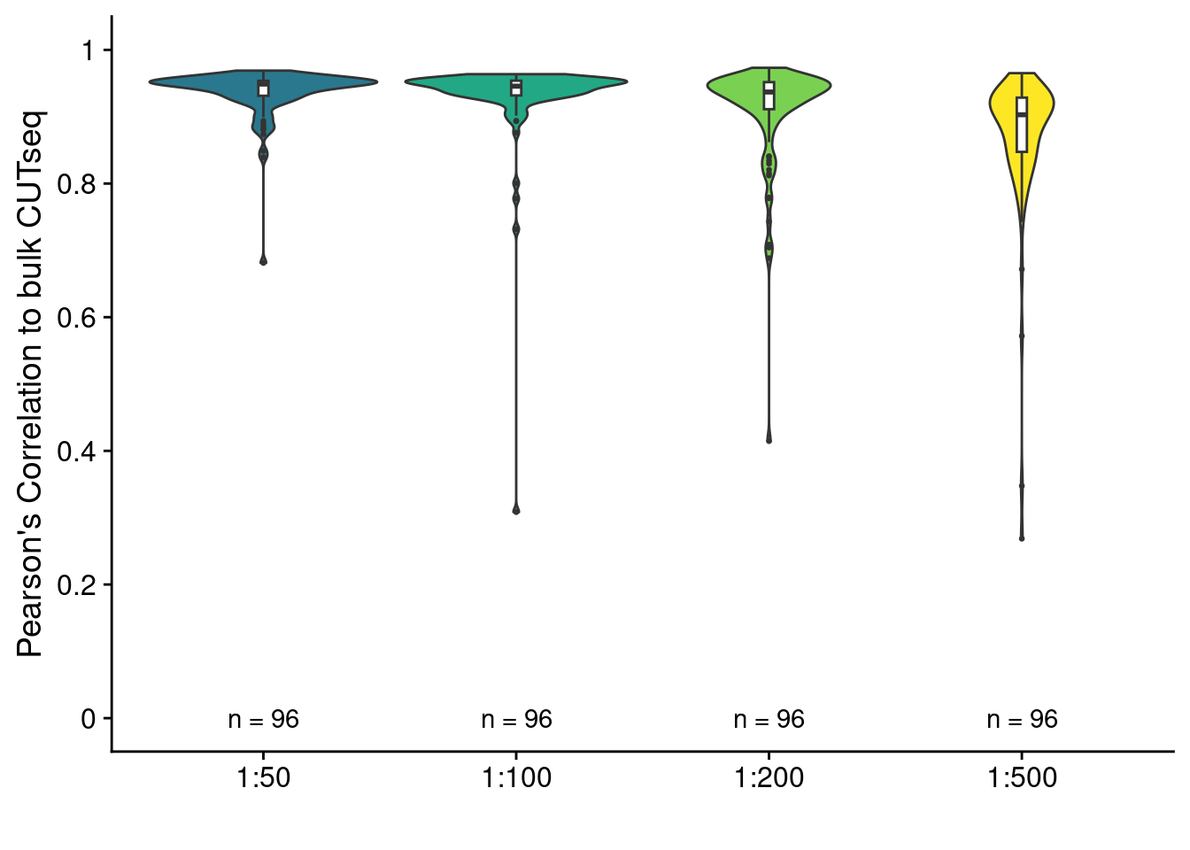
4.3 Representative scCUTseq and sMALBAC profiles of SKBR3 cells
smalbac_profile = readRDS("./data/technical_validation/smalbac_bc221.rds")
scCUTseq_profile = readRDS("./data/technical_validation/scCUTseq_NZ40.rds")

# Plot the profiles
plotProfile(smalbac_profile$segments_read[["NZ58"]], smalbac_profile$counts_gc[["NZ58"]], smalbac_profile$bins)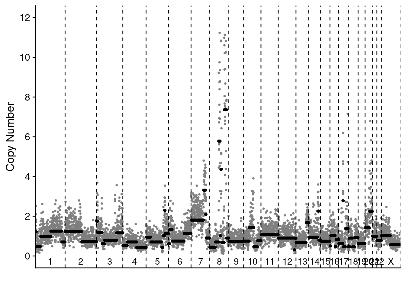
plotProfile(scCUTseq_profile$segments_read[["ACTGAGAT"]], scCUTseq_profile$counts_gc[["ACTGAGAT"]], scCUTseq_profile$bins)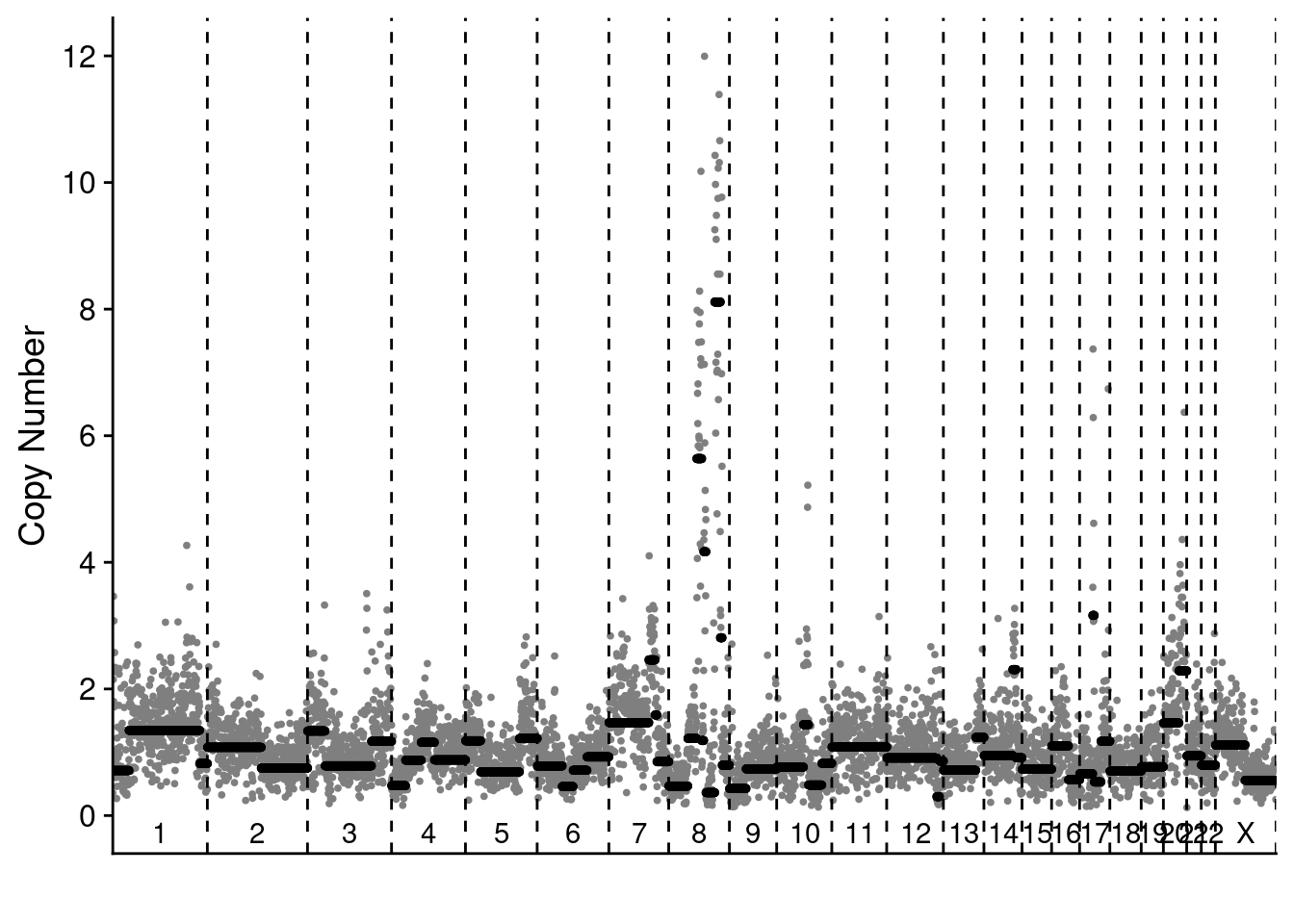
4.4 Lorenz curves of (sc)CUTseq and (scaled) MALBAC
Lorenz curves of Bulk CUTseq, MALBAC (fixed), MALBAC (live), sMALBAC (fixed), sMALBAC (live) and two fixed scCUTseq cells
raw = readRDS("./data/technical_validation/lorenz-counts-500kb.rds")

# Give names
setnames(raw, c("NEBNext - live 1:1", "NEBNext - fixed 1:1", "NEBNext - live 1:200",
                "NEBNext - fixed 1:200", "scCUTseq - Cell 1", "scCUTseq - Cell 2", "Bulk CUTseq"))

lorenz = lapply(colnames(raw), function(sample) {
  # Get lorenz curve points
  lc = Lc(raw[[sample]])

  return(data.table(l = lc$L, p = lc$p, sample = sample))
})

lorenz = rbindlist(lorenz)

ggplot(lorenz, aes(x = p, y = l, color = sample)) +
  geom_abline(slope = 1, size = 1.25) +
  geom_path(aes(group = sample), size = 1.25) +
  scale_y_continuous(expand = c(0, 0)) +
  scale_x_continuous(expand = c(0, 0)) +
  scale_color_npg() +
  labs(y = "Cumulative fraction of total reads",
       x = "Cumulative fraction of genome", color = "") +
  coord_equal()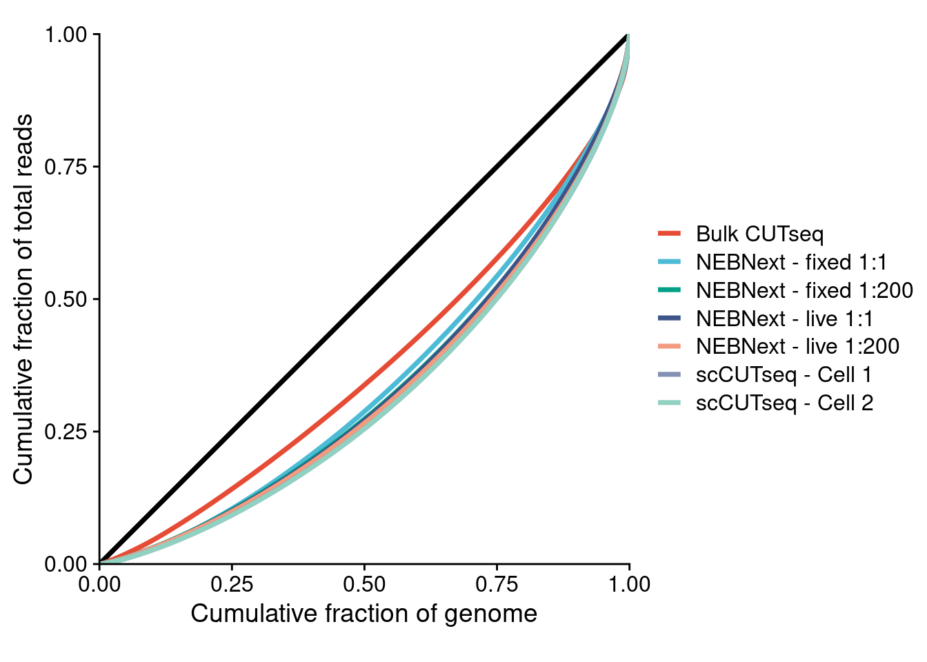
4.5 Pearson correlation of fixed versus live SKBR3 cells
Pearson correlation of fixed and live SKBR3 libraries prepared with either scaled down (1:200) MALBAC or standard MALBAC followed by commercial library preparation.
files = c("./data/technical_validation/smalbac_bc221.rds",
          "./data/technical_validation/malbac_bc229.rds")

total = lapply(files, function(i) {
  rds = readRDS(i)
  return(rds$copynumber)
})

dt = do.call(cbind, total)

setnames(dt, c("MALBAC 1:200 - fixed (cell 3)", "MALBAC 1:200 - live (cell 1)",
               "MALBAC 1:200 - fixed (cell 1)", "MALBAC 1:200 - live (cell 2)",
               "MALBAC 1:200 - live (cell 3)", "MALBAC 1:200 - fixed (cell 2)",
               "MALBAC 1:1 - live (cell 4)", "MALBAC 1:1 - fixed (cell 4)",
               "MALBAC 1:1 - fixed (cell 2)", "MALBAC 1:1 - live (cell 1)",
               "MALBAC 1:1 - fixed (cell 3)", "MALBAC 1:1 - fixed (cell 1)",
               "MALBAC 1:1 - live (cell 3)", "MALBAC 1:1 - live (cell 2)"))

# Plot correlations
res = cor(dt)

res_m = reshape2::melt(res, na.rm = T)
setDT(res_m)

res_m = res_m[grepl("live", Var1) & grepl("fixed", Var2), ]
res_m[, Var1 := factor(Var1, levels = c("MALBAC 1:200 - live (cell 1)", "MALBAC 1:200 - live (cell 2)",
                                        "MALBAC 1:200 - live (cell 3)", "MALBAC 1:1 - live (cell 1)",
                                        "MALBAC 1:1 - live (cell 2)", "MALBAC 1:1 - live (cell 3)",
                                        "MALBAC 1:1 - live (cell 4)"))]
res_m[, Var2 := factor(Var2, levels = rev(c("MALBAC 1:200 - fixed (cell 1)", "MALBAC 1:200 - fixed (cell 2)",
                                            "MALBAC 1:200 - fixed (cell 3)", "MALBAC 1:1 - fixed (cell 1)",
                                            "MALBAC 1:1 - fixed (cell 2)", "MALBAC 1:1 - fixed (cell 3)",
                                            "MALBAC 1:1 - fixed (cell 4)")))]

ggplot(res_m, aes(x = Var1, y = Var2, fill = value)) +
  geom_tile() +
  scale_y_discrete("") +
  scale_x_discrete("", position = "top") +
  geom_text(aes(label = round(value, 3))) +
  scale_fill_viridis("Pearson's\ncorrelation", option="B", begin = 0.75, direction = -1) +
  theme(axis.text.x = element_text(angle = 45, hjust = 0, vjust = 0.5),
        axis.line = element_blank())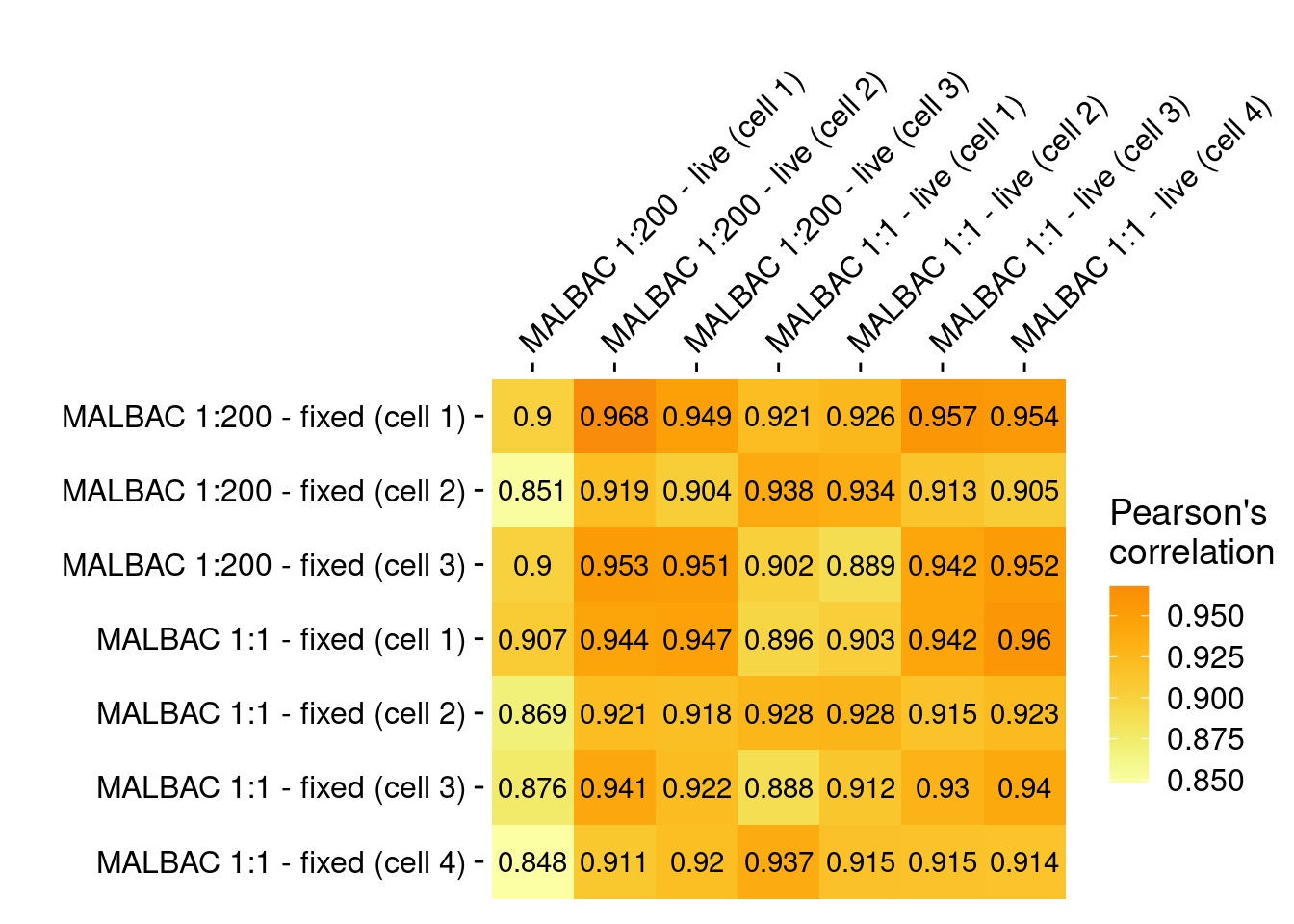
4.6 Genomewide copy number profiles of cell lines
Heatmap of genomewide copy number profiles of SKBR3 (live and fixed), IMR90 and MCF10A cell lines
# Read in cnv.rds and extract HQ profiles
cn = readRDS("./data/technical_validation/cell_lines_heatmap.rds")

# Get annotation
annot = data.table(samples = factor(colnames(cn[, 4:ncol(cn)])),
                   variable = "cell_type",
                   value = gsub("-.*", "", colnames(cn[, 4:ncol(cn)])))

# Plot heatmap
plotHeatmap(cn[, 4:ncol(cn)], cn[, 1:3], annotation = annot, linesize = 2)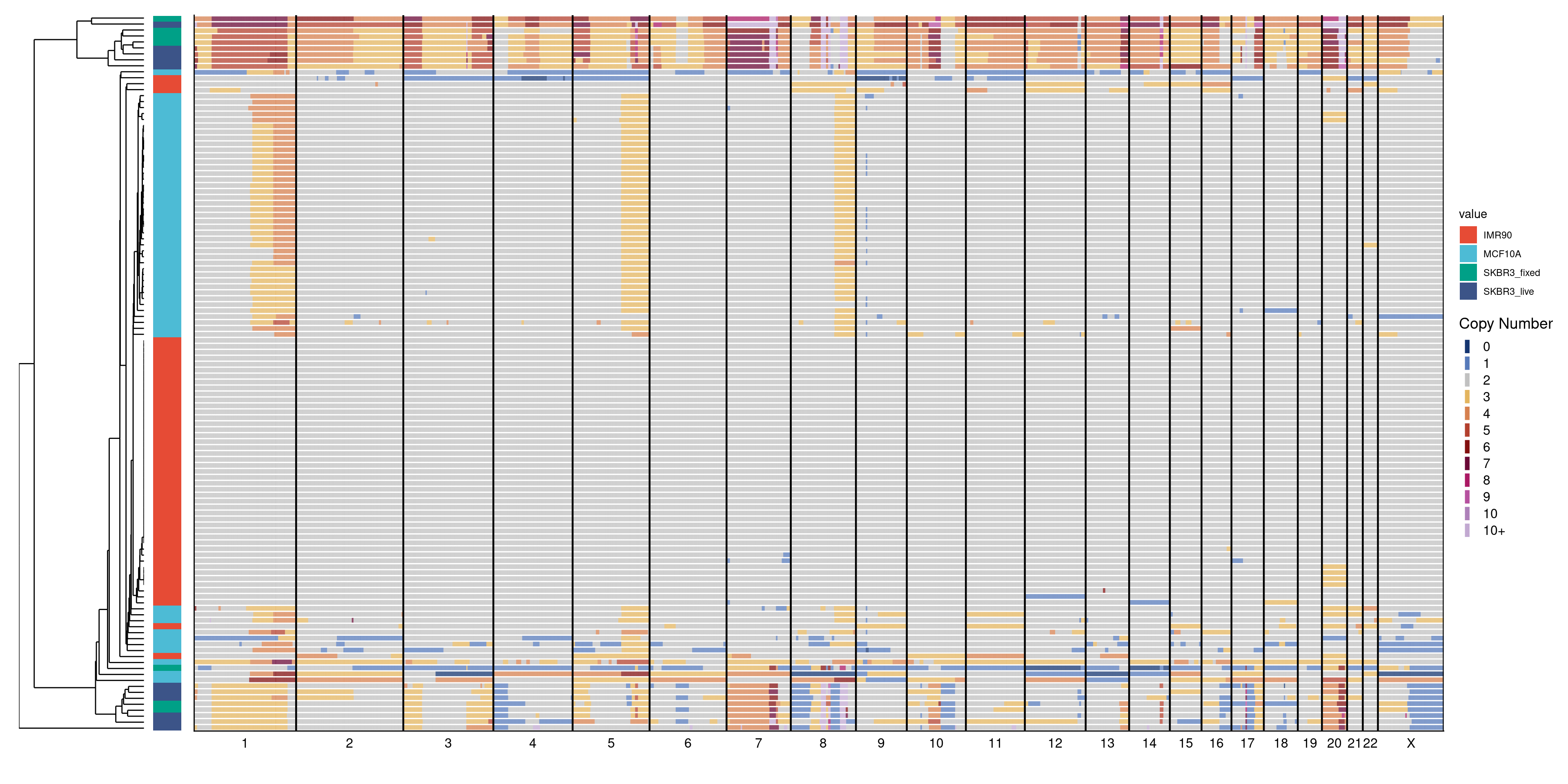
4.7 Cross-contamination experiment with Dm and Hs
# Load in total number of reads (pre and post deduplication)
counts = readRDS("./data/technical_validation/hs_dm_counts.rds")

# Melt datatable
counts = melt(counts)

# Format for plotting
counts[, value := value / 1e6]
counts[, cell := gsub(" POS", "", cell)]
counts[, replicate := gsub(".*_", "", variable)]
counts[, variable := gsub("_rep.*", "", variable)]
counts[, variable := factor(variable, levels = c("all_hs", "all_dm"))]

ggplot(counts, aes(x=variable, y=value, color = cell)) +
  geom_boxplot(outlier.shape = NA) +
  geom_point(position = position_jitterdodge(jitter.width = .2)) +
  facet_wrap(~replicate) +
  labs(y = "Reads per cell (M)",
       x = "",
       color = "") +
  scale_color_manual(values = brewer.pal(4, "Set1")) +
  theme(legend.position = "top")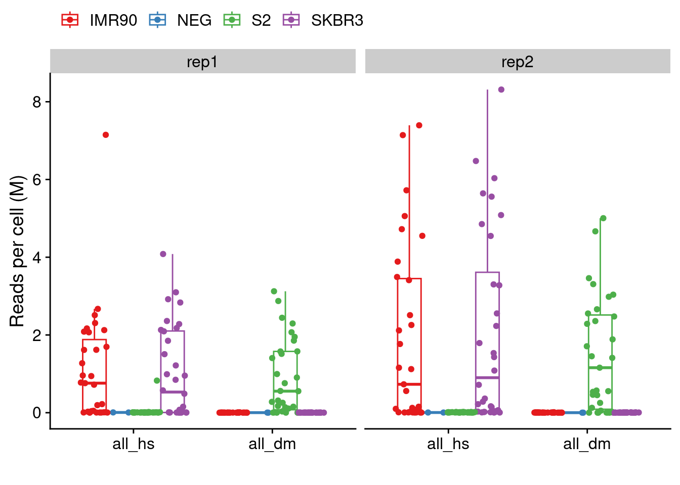
4.8 Detection of CRISPR induced deletions
Select cells that have some type of alteration in the CRISPR area and then plot a zoom-in heatmap of this region.
# Load TK6 data
treated = readRDS("./data/TK6_treated.rds")
untreated = readRDS("./data/TK6_untreated.rds")

# Set bins
bins = treated[, 1:3]

# Set region of interest for heatmap
roi = data.table(chr = "11", start = 118307205, end = 125770541) # This is the CRISPR targeted region
roi_bins = foverlaps(roi, bins, which = T)$yid

# Select cells that have any part of the ROI altered (cells of interest; COI)
treated_coi = unlist(sapply(colnames(treated[, 4:ncol(treated)]), function(x) {
  count = sum(treated[roi_bins, ..x] != 2)
  if(count > 2) return(x)
}))

untreated_coi = unlist(sapply(colnames(untreated[, 4:ncol(untreated)]), function(x) {
  count = sum(untreated[roi_bins, ..x] != 2)
  if(count > 2) return(x)
}))

# Get bins of -10mb and +10 mb of gRNAs
closest = data.table(chr = "11", start = c(roi$start[1] - 1e7, roi$end[1] + 1e7))
setkey(closest, chr, start)
plot_window = bins[closest, roll = "nearest"]
zoom_index = which(bins$chr == plot_window[1, chr] & bins$start >= plot_window[1, start] & bins$end <= plot_window[2, end])

# Subset data on both samples and genomic region
total = cbind(treated[zoom_index, ..treated_coi], untreated[zoom_index, ..untreated_coi])
bins = bins[zoom_index]

# Make annotation data table
annot = data.table(sample = c(treated_coi, untreated_coi),
                   variable = "condition",
                   value = c(rep("treated", length(treated_coi)), rep("untreated", length(untreated_coi))))

# Plot heatmap
plotHeatmap(total, bins, annotation = annot, linesize = 2)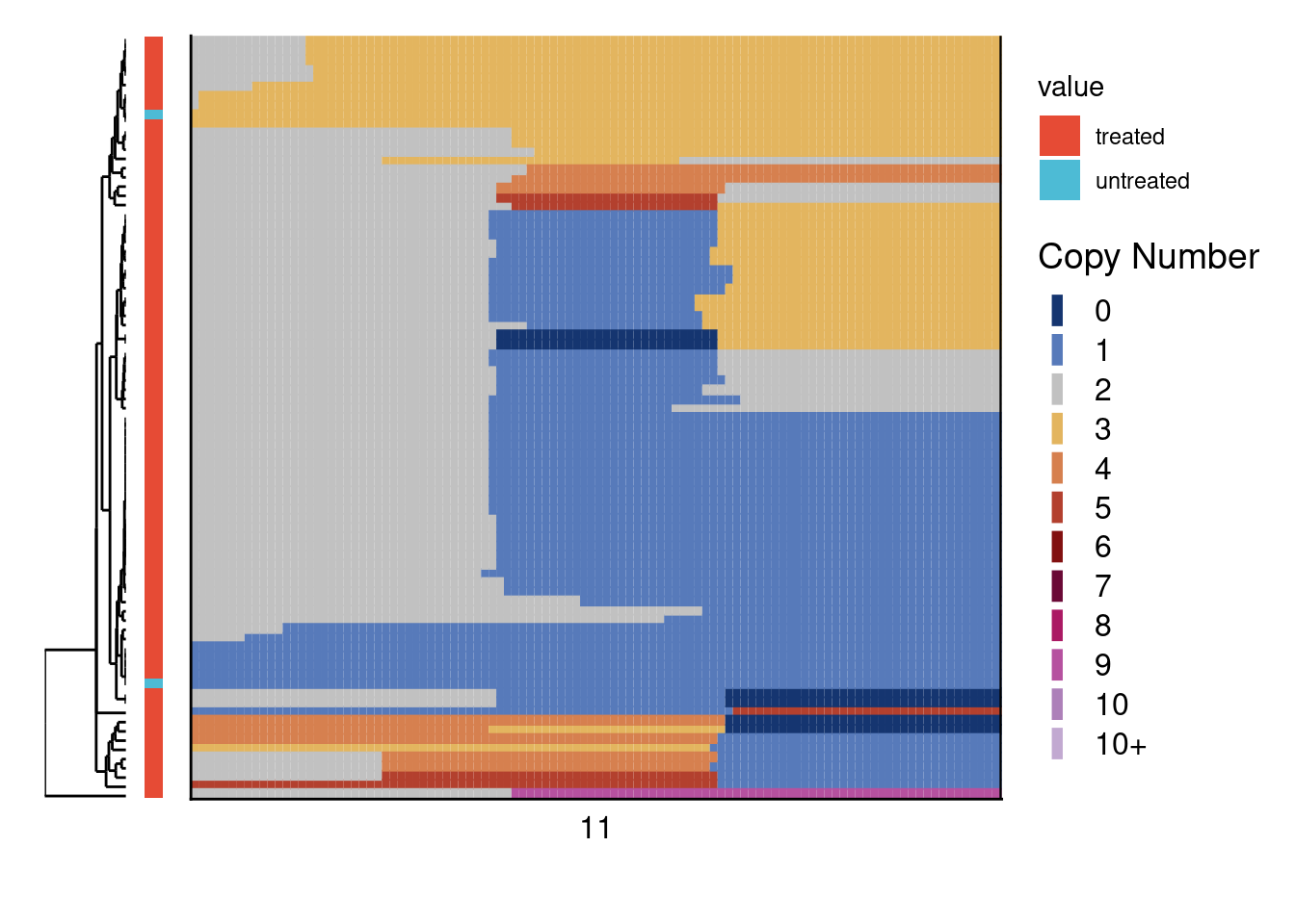
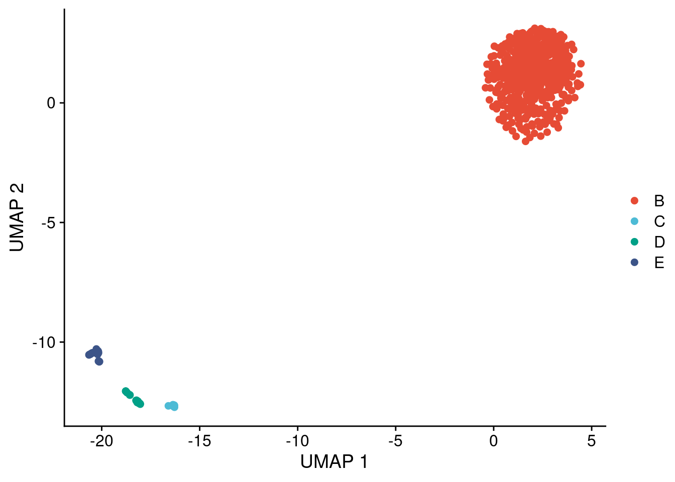
Plot UMAPs of chromosome 11 copy number profiles. Take note that we did not set a seed for this analysis, so the UMAP can look slightly different than the figure we show. The differences are minimal and do not change any of the conclusions we draw from these plots.
dt = merge(treated, untreated, by = c("chr", "start", "end"))

# Make UMAP dataframe only using chr 11 profiles
total_umap = umap(t(dt[chr == "11", 4:ncol(dt)]), n_neighbors = 24, spread = 1, min_dist = 0)
umap_dt = data.table(x = total_umap[, 1],
                     y = total_umap[, 2],
                     sample = colnames(dt[, 4:ncol(dt)]),
                     group = ifelse(colnames(dt[, 4:ncol(dt)]) %in% colnames(treated), "Treated", "Untreated"))

# Plot UMAP
ggplot(umap_dt, aes(x = x, y = y, color = group)) +
  geom_point(size = 1.5) +
  scale_color_npg() +
  labs(x  = "UMAP 1", y = "UMAP 2", color = "")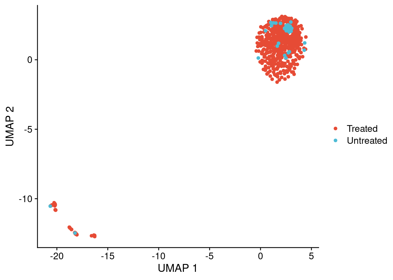
# Cluster UMAP using DBSCAN
clones = dbscan::hdbscan(umap_dt[,c(1:2)],
                         minPts = 9)
umap_dt[, clone := LETTERS[clones$cluster + 1]]

# Plot clusters
ggplot(umap_dt, aes(x = x, y = y, color = clone)) +
  geom_point(size = 2) +
  scale_color_npg() +
  labs(x  = "UMAP 1", y = "UMAP 2", color = "")