19 COSMIC deletions and targeted panel mutations
This sections produces all the figures used in Supplementary Figure 19.
19.1 TRR/FER specific subclones
First we look at subclones (identified based on copynumber profiles previously) that are exclusively present in Tumour-Rich Regions (TRRs) or Focally Enriched regions (FERs). For these subclones we plot the genes that are altered. The spatial distributions of cells from these subclones can be found in the plots created previously (scCUTseq_subclone-distributions.Rmd).
profiles = fread("./data/subclones/P6_median_cn.tsv")
clones = fread("./data/subclones/P6_clones.tsv")
cosmic = fread("./data/genelists/cosmic_gene-census.tsv")
annot = fread("./annotation/P6.tsv", header = F)

# Merge clones with annot
clones[, library := gsub("_.*", "", sample_id)]
clones_annot = merge(clones, annot, by.x = "library", by.y = "V1")

# Select clones that are only present in cancer/focal
total = clones_annot[, .(paste(unique(V3), collapse = ";")), by = cluster]

clones_selected = total[!grepl("Normal", V1)]

# Get selected
profiles = profiles[cluster %in% clones_selected$cluster]
profiles = profiles[(total_cn != 2 & chr != "X") | (total_cn != 1 & chr == "X")]

# Get overlaps
setkey(profiles, chr, start, end)
setkey(cosmic, chr, start, end)
overlaps = foverlaps(cosmic, profiles)[!is.na(total_cn)]
overlaps[, alteration := ifelse(total_cn < 2, "Deleted", "Amplified")]

# Get unique
unique_overlaps = unique(overlaps[, .(name, gene, alteration)])

# Make oncoprint
unique_overlaps_wide = dcast(unique_overlaps, name ~ gene, value.var = "alteration")
mat = as.matrix(unique_overlaps_wide[, 2:ncol(unique_overlaps_wide)])
rownames(mat) = unique_overlaps_wide$name

# Plot oncoprint
# colors
cols = brewer.pal(3, "Set1")[c(1, 2)]
names(cols) = c("Amplified", "Deleted")

oncoPrint(t(mat),
          alter_fun = list(
            background = alter_graphic("rect", width = 0.9, height = 0.9, fill = "#FFFFFF", col = "black", size = .1),
            Amplified = alter_graphic("rect", width = 0.85, height = 0.85, fill = cols["Amplified"]),
            Deleted = alter_graphic("rect", width = 0.85, height = 0.85, fill = cols["Deleted"])),
          col = cols, border = "black", show_column_names = T, show_row_names = T, remove_empty_rows = T,
          show_pct = F, row_names_gp = gpar(fontsize = 17), column_names_gp = gpar(fontsize = 22))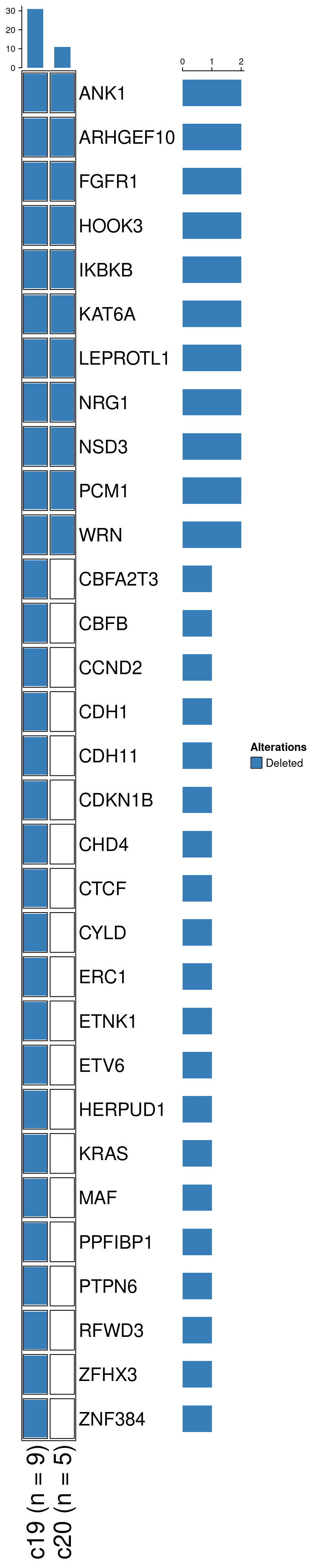
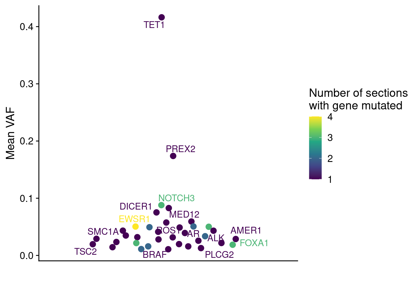
19.2 Variant allele frequency SNVs
Next we wanted to see the distribution of the Variant Allele Frequencies in both of our patients. First we plot P3.
# Load in SNV data
snv = fread("./data/mutations/P3_filtered_SNVs.tsv")

# Remove underscore in sample
snv[, SAMPLE := gsub("_", "", SAMPLE)]

# Remove LOC/2nd genes
snv[, GeneName := gsub("LOC.*:", "", GeneName)]
snv[, GeneName := gsub(":.*", "", GeneName)]

# Get VAFs
muts_vaf = snv[, .(mean_vaf = mean(VAF), count = .N), by = GeneName]

# Plot
ggplot(muts_vaf, aes(x = "", y = mean_vaf, label = GeneName, color = count)) +
  geom_quasirandom(size = 3) +
  geom_text_repel(position = position_quasirandom()) +
  scale_color_viridis_c(name = "Number of sections\nwith gene mutated", option = "D") +
  labs(y = "Mean VAF", x = "", color = "Number of sections\nwith gene mutated") +
  theme(axis.ticks.x = element_blank())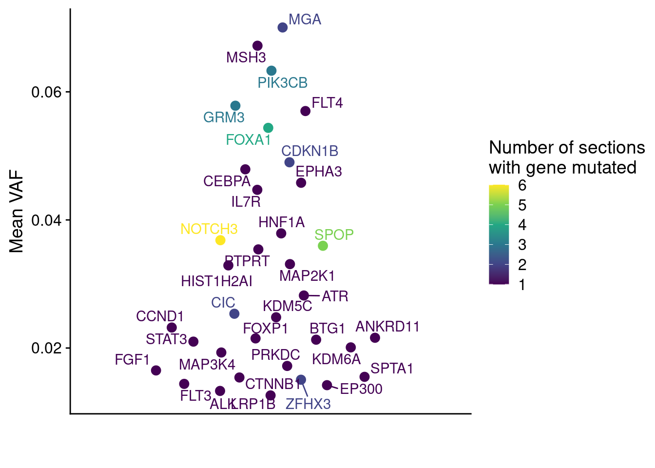
Following this, we do the same for P6.
# Load in SNV data
snv = fread("./data/mutations/P6_filtered_SNVs.tsv")

# Remove underscore in sample
snv[, SAMPLE := gsub("_", "", SAMPLE)]

# Remove LOC/2nd genes
snv[, GeneName := gsub("LOC.*:", "", GeneName)]
snv[, GeneName := gsub(":.*", "", GeneName)]

# Get VAFs
muts_vaf = snv[, .(mean_vaf = mean(VAF), count = .N), by = GeneName]

# Plot
ggplot(muts_vaf, aes(x = "", y = mean_vaf, label = GeneName, color = count)) +
  geom_quasirandom(size = 3) +
  geom_text_repel(position = position_quasirandom()) +
  scale_color_viridis_c(name = "Number of sections\nwith gene mutated", option = "D") +
  labs(y = "Mean VAF", x = "", color = "Number of sections\nwith gene mutated") +
  theme(axis.ticks.x = element_blank())