12 Clonal analysis pseudo-diploid cells
This section produces all the figures used for Figure 2.
# Source setup file
source("./functions/setup.R")

# Load functions
source("./functions/plotHeatmap.R")
12.1 Running MEDICC2
To run MEDICC2 on the pseudo-diploid cells we have to prepare the data. We won’t save this table here, but you can save this and use this as input for MEDICC2. We only show how to run this for P3, but this is the exact same for P6, simply change the input while you load in the data. Because these steps take some time, we don’t actually run this (eval = FALSE) in this Rmarkdown file.
# Load in data
dt = readRDS("./data/P3_pseudodiploid_500kb.rds")

# Melt
dt_m = melt(dt, id.vars = c("chr", "start", "end"))

# Reduce data table
dt_short = dt_m[, as.data.table(reduce(IRanges(start, end))), by = .(chr, variable, value)]
dt_short = dcast(dt_short, chr + start + end + width ~ variable)

# Fill NAs
dt_short = dt_short %>%
  group_by(chr) %>%
  fill(names(.), .direction = "updown") %>%
  ungroup() %>%
  setDT()

# Add diploid
dt_short[, diploid := 2]
dt_short[chr == "X", diploid := 1]

# Get unique start/end sites (unique based on start site) and go back to long format
dt_final = unique(dt_short, by = c("chr", "start"))
dt_final = melt(dt_final, id.vars = c("chr", "start", "end", "width"))
setnames(dt_final, c("chrom", "start", "end", "width", "sample_id", "total_cn"))

# Rename chromosomes
dt_final[chrom == "X", chrom := 23]
dt_final[, chrom := paste0("chr", chrom)]
After we prepared the input for MEDICC2 we can run it. This is down using the following command:
12.2 Plot MEDICC2 results
After running MEDICC2 we can plot the tree that has been generated alongside the scCUTseq genomewide heatmaps. We load in the previously generated input data and the phylogenetic Newick tree from MEDICC2. First we do this for P3.
# Load in data
profiles = fread("./data/phylotrees/P3_input.tsv")
tree = read.tree("./data/phylotrees/P3_500kb.new")

# Reorder profiles
dt = dcast(profiles, chrom + start + end ~ sample_id)
dt = dt[gtools::mixedorder(chrom),]

# Rename chromosomes
setnames(dt, "chrom", "chr")
dt[chr == "chr23", chr := "chrX"]

# Plot tree
tree_plot = ggtree(tree)

# Plot heatmap
col_order = rev(get_taxa_name(tree_plot))
heatmap = plotHeatmap(dt[, 4:ncol(dt)], dt[, 1:3], dendrogram = F, order = col_order, linesize = .75)

# Combine plots
tree_plot + heatmap + plot_layout(widths = c(1, 3))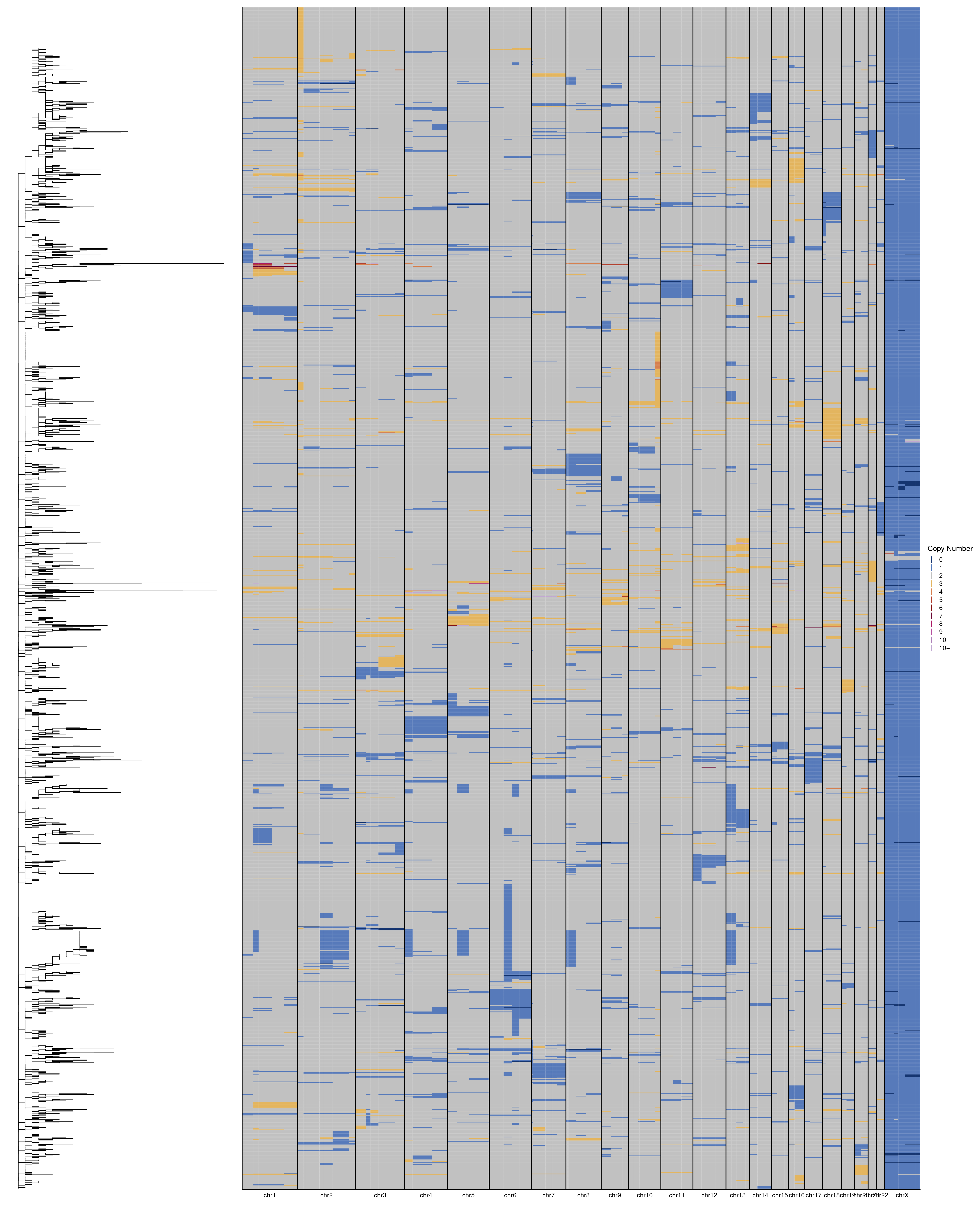
Repeat for P6.
# Load in data
profiles = fread("./data/phylotrees/P6_input.tsv")
tree = read.tree("./data/phylotrees/P6_500kb.new")

# Reorder profiles
dt = dcast(profiles, chrom + start + end ~ sample_id)
dt = dt[gtools::mixedorder(chrom),]

# Rename chromosomes
setnames(dt, "chrom", "chr")
dt[chr == "chr23", chr := "chrX"]

# Plot tree
tree_plot = ggtree(tree)

# Plot heatmap
col_order = rev(get_taxa_name(tree_plot))
heatmap = plotHeatmap(dt[, 4:ncol(dt)], dt[, 1:3], dendrogram = F, order = col_order, linesize = .75)

# Combine plots
tree_plot + heatmap + plot_layout(widths = c(1, 3))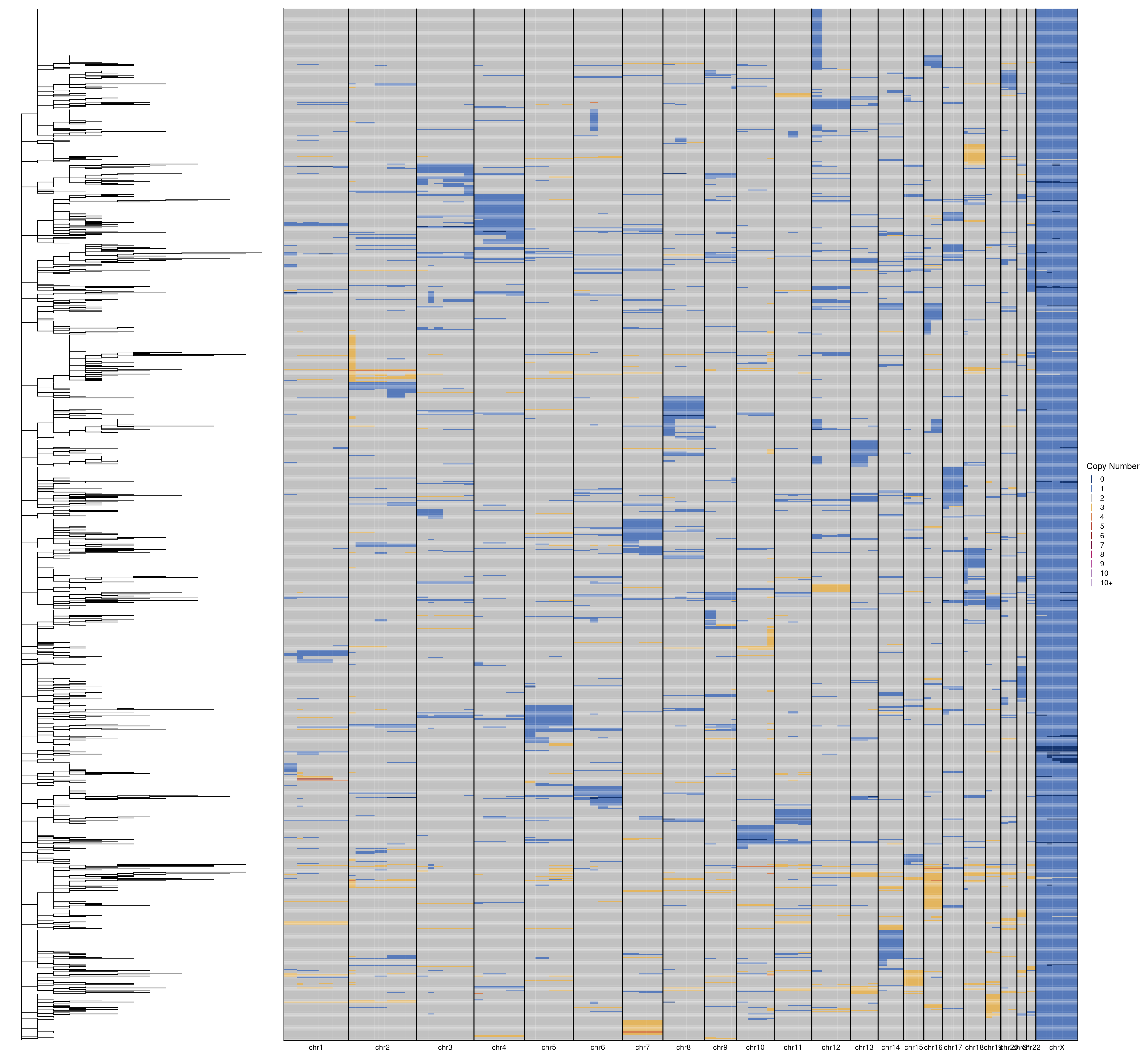
12.3 Identify tumour subclones
After we generated the phylogenetic tree using MEDICC2, we perform clustering upon this tree. To do this we run TreeCluster. We run the following commands for P3 and P6, respectively.
TreeCluster.py -i {input_newick_tree_P3} -t 3 -m max -o {output_clusters_P3} # These are the parameters for P3
TreeCluster.py -i {input_newick_tree_P6} -t 4 -m max -o {output_clusters_P6} # These are the parameters for P6
Next, we want to get the median copy number profile for each subclone. Sometimes it happens that there will be two subclones identified that will have the exact same median copy number profiles, if this is the case, we merge them together. Furthermore, we exclude any subclone that has fewer than 5 cells. The final list of the cell_ids and associated subclone and median copynumber profiles per subclone can be find in the ./data/subclones/ folder.
12.4 Calculate SCNAs per subclones
Calculate the percentage of the genome that is altered for P3.
profiles = fread("./data/subclones/P3_median_cn.tsv")

# Get percentage of AMP/DEL/NEUTRAL
profiles = dcast(profiles, chr + start + end ~ cluster, value.var = "total_cn")
clones = colnames(profiles[, 4:ncol(profiles)])

res = lapply(clones, function(clone) {
  # Without X
  amp_sum = sum(profiles[chr != "X", ..clone] > 2)
  del_sum = sum(profiles[chr != "X", ..clone] < 2)
  neut_sum = sum(profiles[chr != "X", ..clone] == 2)

  # With X
  amp_sum = amp_sum + sum(profiles[chr == "X", ..clone] > 1)
  del_sum = del_sum + sum(profiles[chr == "X", ..clone] < 1)
  neut_sum = neut_sum + sum(profiles[chr == "X", ..clone] == 1)

  return(data.table(clone = clone,
                    gain = amp_sum / nrow(profiles),
                    loss = del_sum / nrow(profiles),
                    neutral = neut_sum / nrow(profiles)))
})

# Rbind results
results = rbindlist(res)
results_m = melt(results, id.vars = "clone")

# Remove n =
results_m[, clone := gsub(" .*", "", clone)]

# Set factor order
results_m[, variable := factor(variable, levels = c("gain", "neutral", "loss"))]
results_m[, clone := factor(clone, levels = gtools::mixedsort(unique(clone)))]

# Plot
ggplot(results_m, aes(x = clone, y = value, fill = variable)) +
  geom_col(color = "black") +
  scale_fill_manual(values = c("neutral" = "white",
                               "gain" = "firebrick3",
                               "loss" = "steelblue"),
                    label = c("loss",
                              "neutral",
                              "gain"),
                    breaks = c("loss",
                               "neutral",
                               "gain")) +
  scale_y_continuous(expand = c(0, 0)) +
  scale_x_discrete(expand = c(0, 0)) +
  labs(y = "Percentage of genome", x = "", fill = "") +
  theme(axis.text.x = element_text(angle = 45, hjust = 1, vjust = 1)) +
  coord_flip()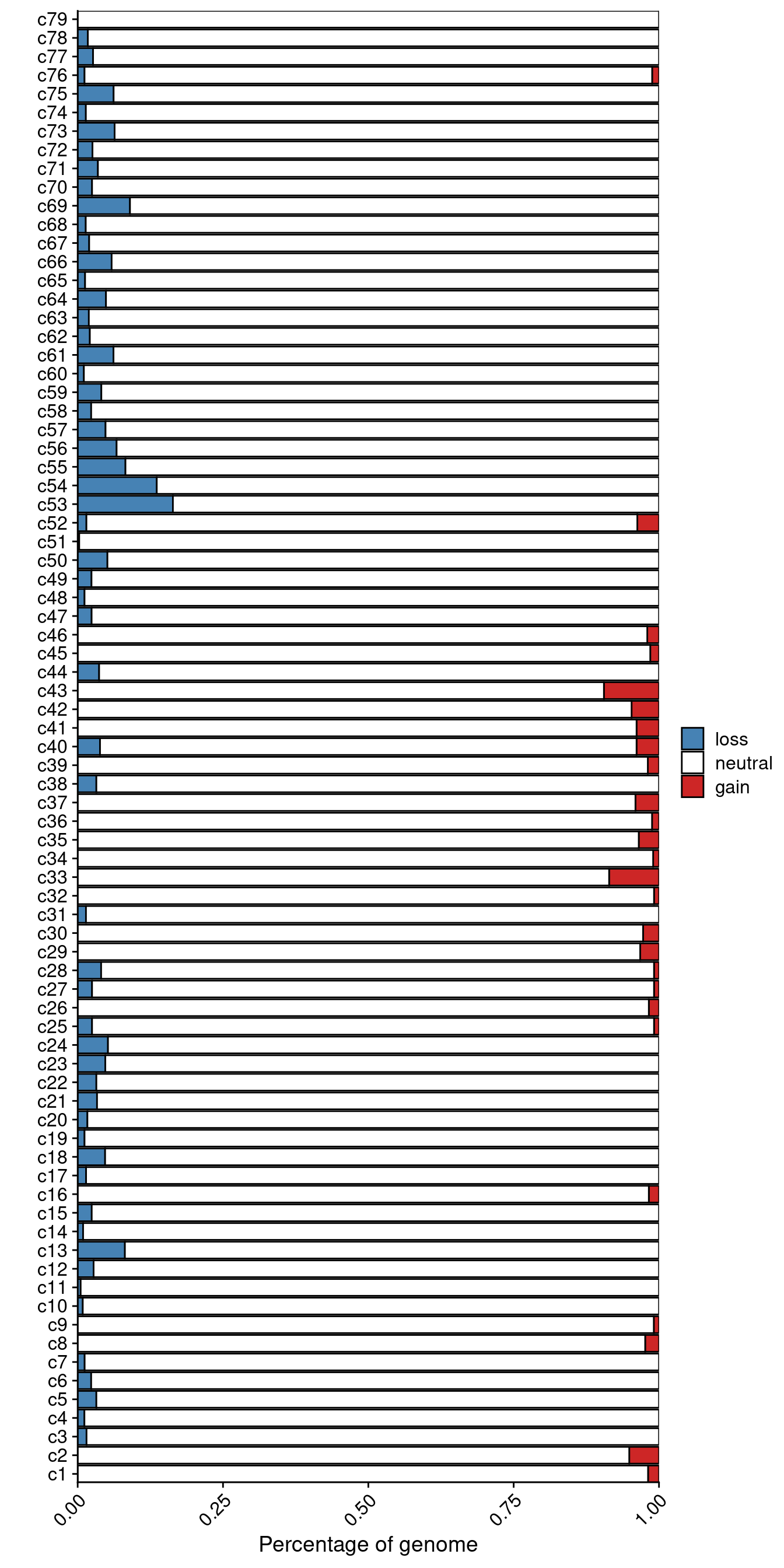
Calculate the percentage of the genome that is altered for P6.
profiles = fread("./data/subclones/P6_median_cn.tsv")

# Get percentage of AMP/DEL/NEUTRAL
profiles = dcast(profiles, chr + start + end ~ cluster, value.var = "total_cn")
clones = colnames(profiles[, 4:ncol(profiles)])

res = lapply(clones, function(clone) {
  # Without X
  amp_sum = sum(profiles[chr != "X", ..clone] > 2)
  del_sum = sum(profiles[chr != "X", ..clone] < 2)
  neut_sum = sum(profiles[chr != "X", ..clone] == 2)

  # With X
  amp_sum = amp_sum + sum(profiles[chr == "X", ..clone] > 1)
  del_sum = del_sum + sum(profiles[chr == "X", ..clone] < 1)
  neut_sum = neut_sum + sum(profiles[chr == "X", ..clone] == 1)

  return(data.table(clone = clone,
                    gain = amp_sum / nrow(profiles),
                    loss = del_sum / nrow(profiles),
                    neutral = neut_sum / nrow(profiles)))
})

# Rbind results
results = rbindlist(res)
results_m = melt(results, id.vars = "clone")

# Remove n =
results_m[, clone := gsub(" .*", "", clone)]

# Set factor order
results_m[, variable := factor(variable, levels = c("gain", "neutral", "loss"))]
results_m[, clone := factor(clone, levels = gtools::mixedsort(unique(clone)))]

# Plot
ggplot(results_m, aes(x = clone, y = value, fill = variable)) +
  geom_col(color = "black") +
  scale_fill_manual(values = c("neutral" = "white",
                               "gain" = "firebrick3",
                               "loss" = "steelblue"),
                    label = c("loss",
                              "neutral",
                              "gain"),
                    breaks = c("loss",
                               "neutral",
                               "gain")) +
  scale_y_continuous(expand = c(0, 0)) +
  scale_x_discrete(expand = c(0, 0)) +
  labs(y = "Percentage of genome", x = "", fill = "") +
  theme(axis.text.x = element_text(angle = 45, hjust = 1, vjust = 1)) +
  coord_flip()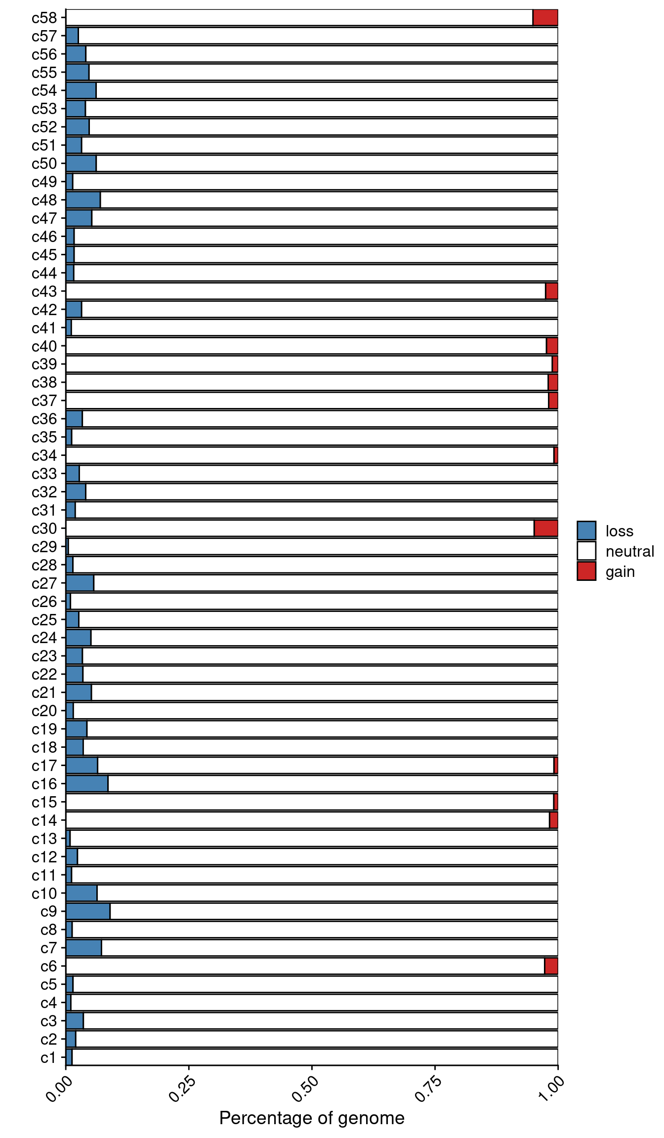
12.5 Calculate entropy per subclone
To assess whether subclones are highly localized in the prostate or widespread we calculate the entropy per subclone. We first normalize the number of cells from each subclone in each section based on the total number of cells that pass QC in that section. Then we calculate the 2D Entropy.
# Load in annotation and clusters and cn profiles
annot = fread("./annotation/P3.tsv",
              header = F, col.names = c("library", "section", "tissue_type"))
clusters = fread("./data/subclones/P3_clones.tsv")

# Get library info and merge
clusters[, library := gsub("_.*", "", sample_id)]
total = merge(clusters, annot, all.x = T)

# Get counts per region and total per region
counts = total[, .N, by = .(section, cluster)]
counts_total = total[, .(total = .N), by = cluster]

# Merge and get fraction of total
counts = merge(counts, counts_total)
counts[, fraction := N / total]
counts[, cluster := as.character(cluster)]

# Add coordinates
counts[, x := as.numeric(gsub("L|C.", "", section))]
counts[, y := as.numeric(gsub("L.|C", "", section))]
counts[, name := paste0(cluster, " (n = ", total, ")")]

# Normalize for total per section
counts_overall = counts[, .(total_cells = sum(N)), by = .(section, x, y)]
counts = merge(counts, counts_overall, by = c("section", "x", "y"))
counts[, normalized_count := N / total_cells]

res = lapply(unique(counts$name), function(clone) {
  # Complete
  dt = counts[name == clone]
  fill_dt = data.table(cluster = gsub("c| .*", "", clone),
                       section = annot[!section %in% dt$section, section],
                       N = NA,
                       fraction = NA,
                       total = unique(dt$total),
                       normalized_count = NA,
                       total_cells = NA,
                       name = clone)
  fill_dt[, x := as.numeric(gsub("L|C.", "", section))]
  fill_dt[, y := as.numeric(gsub("L.|C", "", section))]
  dt = rbind(dt, fill_dt)

  mat = as.matrix(dcast(dt, y~x, value.var = "normalized_count"))
  mat = mat[, 2:ncol(mat)]
  mat[is.na(mat)] = 0
  return(data.table(name = clone, entropy = Entropy(mat)))
})

# Rbind results
result = rbindlist(res)
result[, clone := gsub(" .*", "", name)]
setorder(result, entropy)

# Plot P3
ggplot(result, aes(x = "", y = entropy, label = clone)) +
  geom_quasirandom(size = 5) +
  labs(y = "Entropy", x = "") +
  geom_text_repel(data = result[1:5], size = 5)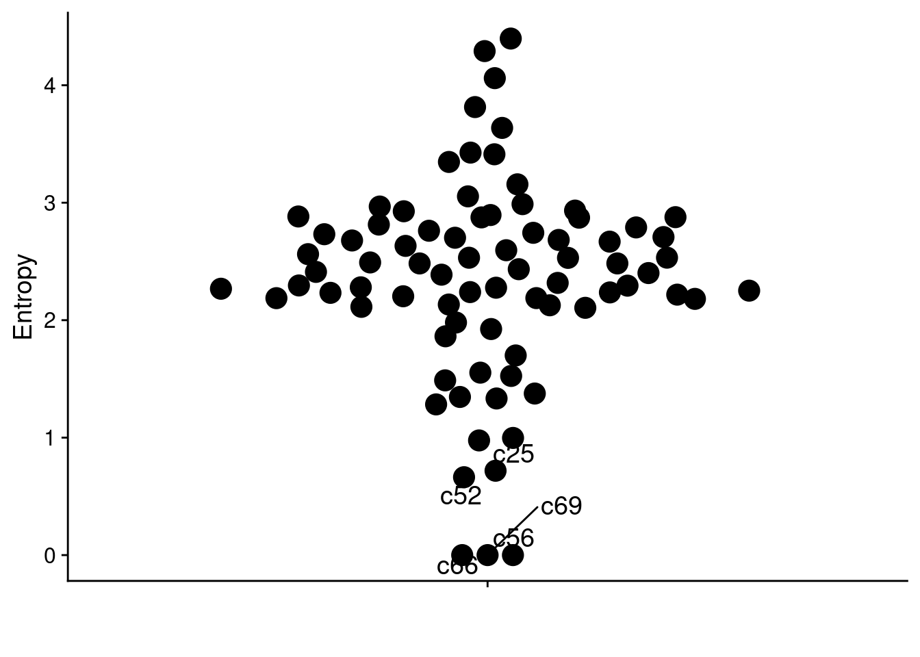
And, once again, repeat this for P6.
# Load in annotation and clusters and cn profiles
annot = fread("./annotation/P6.tsv",
              header = F, col.names = c("library", "section", "tissue_type"))
clusters = fread("./data/subclones/P6_clones.tsv")

# Get library info and merge
clusters[, library := gsub("_.*", "", sample_id)]
total = merge(clusters, annot, all.x = T)

# Get counts per region and total per region
counts = total[, .N, by = .(section, cluster)]
counts_total = total[, .(total = .N), by = cluster]

# Merge and get fraction of total
counts = merge(counts, counts_total)
counts[, fraction := N / total]
counts[, cluster := as.character(cluster)]

# Add coordinates
counts[, x := as.numeric(gsub("L|C.", "", section))]
counts[, y := as.numeric(gsub("L.|C", "", section))]
counts[, name := paste0(cluster, " (n = ", total, ")")]

# Normalize for total per section
counts_overall = counts[, .(total_cells = sum(N)), by = .(section, x, y)]
counts = merge(counts, counts_overall, by = c("section", "x", "y"))
counts[, normalized_count := N / total_cells]

res = lapply(unique(counts$name), function(clone) {
  # Complete
  dt = counts[name == clone]
  fill_dt = data.table(cluster = gsub("c| .*", "", clone),
                       section = annot[!section %in% dt$section, section],
                       N = NA,
                       fraction = NA,
                       total = unique(dt$total),
                       normalized_count = NA,
                       total_cells = NA,
                       name = clone)
  fill_dt[, x := as.numeric(gsub("L|C.", "", section))]
  fill_dt[, y := as.numeric(gsub("L.|C", "", section))]
  dt = rbind(dt, fill_dt)

  mat = as.matrix(dcast(dt, y~x, value.var = "normalized_count"))
  mat = mat[, 2:ncol(mat)]
  mat[is.na(mat)] = 0
  return(data.table(name = clone, entropy = Entropy(mat)))
})

# Rbind results
result = rbindlist(res)
result[, clone := gsub(" .*", "", name)]
setorder(result, entropy)

# Plot P6
ggplot(result, aes(x = "", y = entropy, label = clone)) +
  geom_quasirandom(size = 5) +
  labs(y = "Entropy", x = "") +
  geom_text_repel(data = result[1:5], size = 5)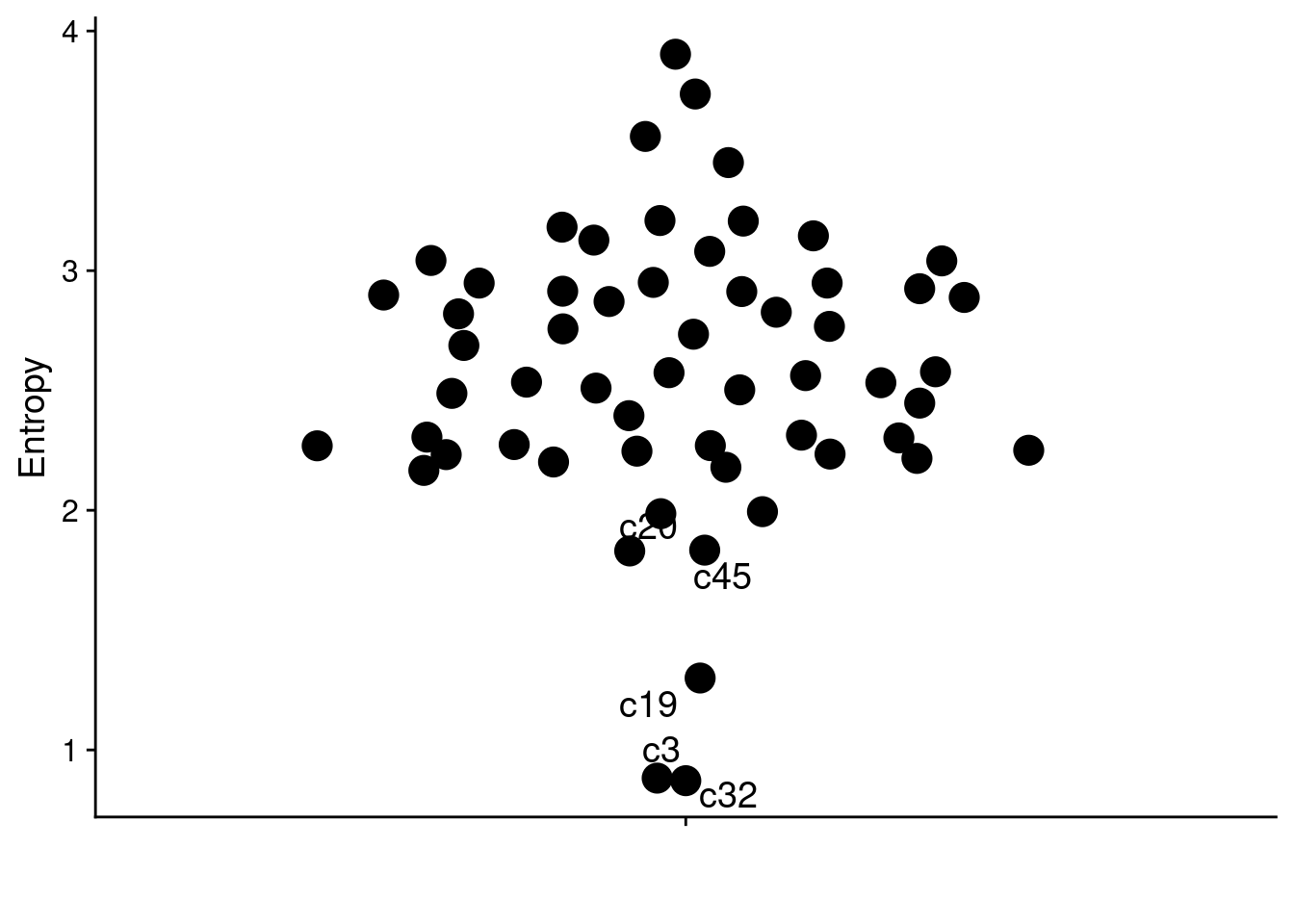
Finally, the heatmaps of the distribution of each subclone (Figure 2k, l), can be found in the Supplementary Figure 12-15 section.