5 Comparison of scCUTseq and ACT
This sections produces all the figures used in Supplementary Figure 3.
We compare the Breadth of Coverage, Overdispersion and overall copynumber profiles between different sections in Patient 3 that were sequenced by both ACT and scCUTseq.
# Source setup file
source("./functions/setup.R")

# Source plotting functions
source("./functions/plotProfile.R")
source("./functions/plotHeatmap.R")
5.1 Calculate breadth of coverage
We downsampled bam files to 800K reads using the following commands in bash and ran our copynumber calling pipeline (described in Preprocessing.Rmd) and use the resulting cnv.rds to get information about cell quality.
samtools view ${INSAMPLEBASE}.bam -H > ${INSAMPLEBASE}.sam&& samtools view $INSAMPLEBASE.bam | shuf -n 800000 --random-source=$INSAMPLEBASE.bam >> $INSAMPLEBASE.sam&& samtools sort -o ../downsampling/bamfiles/$OUTBAM $INSAMPLEBASE.sam&& rm $INSAMPLEBASE.sam&& genomeCoverageBed -ibam ../downsampling/bamfiles/$OUTBAM -fs 50 -max 1 > ../downsampling/coverage/$COVHISTFILEWe then used the $COVHISTFILE output to calculate the breadth of coverage.
# Define BoC function
calc_coverage = function(path) {

  inpaths = Sys.glob(paste0(path, "*.covhist.txt"))

  coverage.stats = tibble(bed_path=inpaths) %>%
    mutate(cellname = str_extract(basename(bed_path), "^[^.]*")) %>%
    group_by(cellname) %>%
    summarize(.groups="keep",
              read_tsv(bed_path,
                       col_names=c("refname", "depth", "count",
                                   "refsize", "frac"),
                       col_types=cols(col_character(), col_double(),
                                      col_double(), col_double(),
                                      col_double())),
    ) %>%
    filter(refname=="genome") %>%
    summarize(breadth = 1 - frac[depth==0],
              .groups="keep")

}

# Calculate BoC on the COVHIST files
sccutseq = calc_coverage("./data/downsampling/coverage/scCUTseq/")
act = calc_coverage("./data/downsampling/coverage/ACT/")

# SetDT
setDT(sccutseq)
setDT(act)

# Load copynumber profiles to get HQ cells
p3 = readRDS("./data/downsampling/P3.rds")
p3_stats = p3$stats
p3_hq = p3_stats[classifier_prediction == "good", sample]

# ACT
CD5p = readRDS("./data/downsampling/CD5p.rds")
CD7p = readRDS("./data/downsampling/CD7p.rds")
CD4p = readRDS("./data/downsampling/CD4p.rds")
CD2p = readRDS("./data/downsampling/CD2p.rds")
CD6p = readRDS("./data/downsampling/CD6p.rds")
CD3p = readRDS("./data/downsampling/CD3p.rds")

act_hq = c(paste0("CD5p_", CD5p$stats[classifier_prediction == "good", sample]),
           paste0("CD7p_", CD7p$stats[classifier_prediction == "good", sample]),
           paste0("CD4p_", CD4p$stats[classifier_prediction == "good", sample]),
           paste0("CD2p_", CD2p$stats[classifier_prediction == "good", sample]),
           paste0("CD6p_", CD6p$stats[classifier_prediction == "good", sample]),
           paste0("CD3p_", CD3p$stats[classifier_prediction == "good", sample]))

# Select HQ samples
sccutseq = sccutseq[cellname %in% p3_hq, ]
act = act[cellname %in% act_hq, ]

# Combine
sccutseq[, tech := "scCUTseq"]
act[, tech := "ACT"]
dt = rbind(sccutseq, act)
dt[, tech := factor(tech, levels = c("scCUTseq", "ACT"))]

# Plot comparison
ggplot(dt, aes(x = tech, y = breadth)) +
  geom_violin() +
  geom_boxplot(width = .15) +
  scale_y_continuous(limits = c(0, 0.0125)) +
  labs(y = "Breadth of coverage", x = "")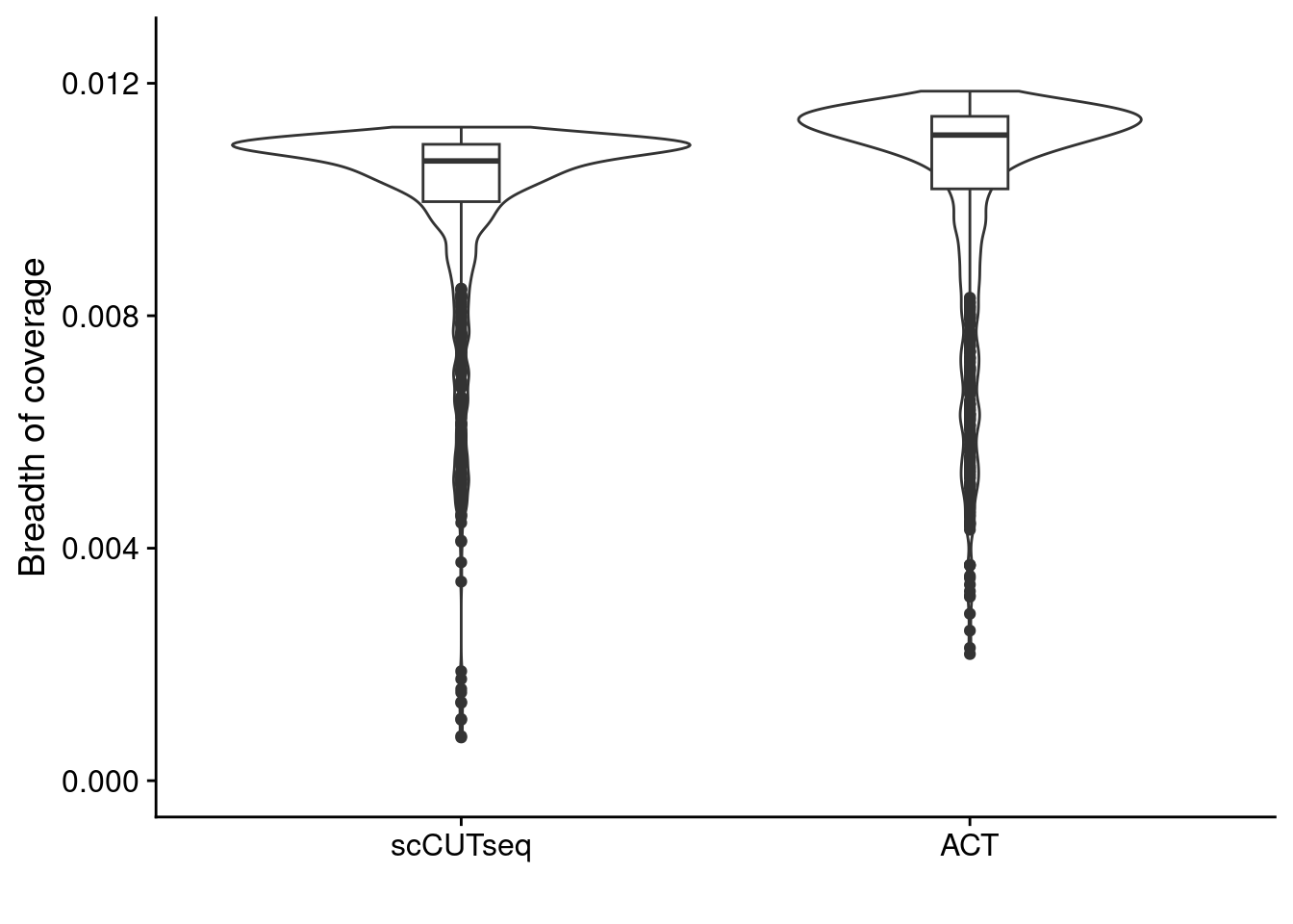
5.2 Calculate overdispersion
Then we used the read counts from each bin to calculate the overdispersion. We also do this on the HQ cells that are selected in the code chunk above.
# Define functions
l2e.normal.sd = function(xs)
{
  # Need at least two values to get a standard deviation
  stopifnot(length(xs) >= 2)
  optim.result = stats::optimize(
    # L2E loss function
    f=function(sd)
      # "Data part", the sample average of the likelihood
      -2 * mean(stats::dnorm(xs, sd=sd)) +
      # "Theta part", the integral of the squared density
      1/(2*sqrt(pi)*sd),
    # Parameter: standard deviation of the normal distribution fit
    interval = c(0, diff(range(xs))))
  return(optim.result$minimum)
}

# A function for estimating the index of dispersion, which is used when
# estimating standard errors for each segment mean
overdispersion = function(v)
{
  # 3 elements, 2 differences, can find a standard deviation
  stopifnot(length(v) >= 3)
  # Differences between pairs of values
  y = v[-1]
  x = v[-length(v)]
  # Normalize the differences using the sum. The result should be around zero,
  # plus or minus square root of the index of dispersion
  vals.unfiltered = (y-x)/sqrt(y+x)
  # Remove divide by zero cases, and--considering this is supposed to be count
  # data--divide by almost-zero cases
  vals = vals.unfiltered[y + x  >= 1]
  # Check that there's anything left
  stopifnot(length(vals) >= 2)
  # Assuming most of the normalized differences follow a normal distribution,
  # estimate the standard deviation
  val.sd = l2e.normal.sd(vals)
  # Square this standard deviation to obtain an estimate of the index of
  # dispersion
  iod = val.sd^2
  # subtract one to get the overdispersion criteria
  iod.over = iod -1
  # normalizing by mean bincounts
  iod.norm = iod.over/mean(v)
  return(iod.norm)
}

# Get count data for scCUTseq and ACT
p3_counts = p3$counts[, p3_stats[classifier_prediction == "good", sample], with = FALSE]
CD5p_counts = CD5p$counts[, CD5p$stats[classifier_prediction == "good", sample], with = FALSE]
CD7p_counts = CD7p$counts[, CD7p$stats[classifier_prediction == "good", sample], with = FALSE]
CD4p_counts = CD4p$counts[, CD4p$stats[classifier_prediction == "good", sample], with = FALSE]
CD2p_counts = CD2p$counts[, CD2p$stats[classifier_prediction == "good", sample], with = FALSE]
CD6p_counts = CD6p$counts[, CD6p$stats[classifier_prediction == "good", sample], with = FALSE]
CD3p_counts = CD3p$counts[, CD3p$stats[classifier_prediction == "good", sample], with = FALSE]

# Combine act
act_counts = do.call(cbind, list(CD5p_counts, CD4p_counts, CD2p_counts,
                                 CD7p_counts, CD6p_counts, CD3p_counts))

# Calculate overdispersion
p3_overdispersion = lapply(p3_counts, function(x) {
  overdispersion(x)
})

act_overdispersion = lapply(act_counts, function(x) {
  overdispersion(x)
})

# Make into DT
act_dt = data.table(method = "ACT", overdispersion = unlist(act_overdispersion))
p3_dt = data.table(method = "scCUTseq", overdispersion = unlist(p3_overdispersion))

# Combine DTs
dt = rbind(act_dt, p3_dt)
dt[, method := factor(method, levels = c("scCUTseq", "ACT"))]

# Plot comparison
ggplot(dt, aes(x = method, y = overdispersion)) +
  geom_violin() +
  geom_boxplot(width = .075) +
  labs(y = "Overdispersion", x = "")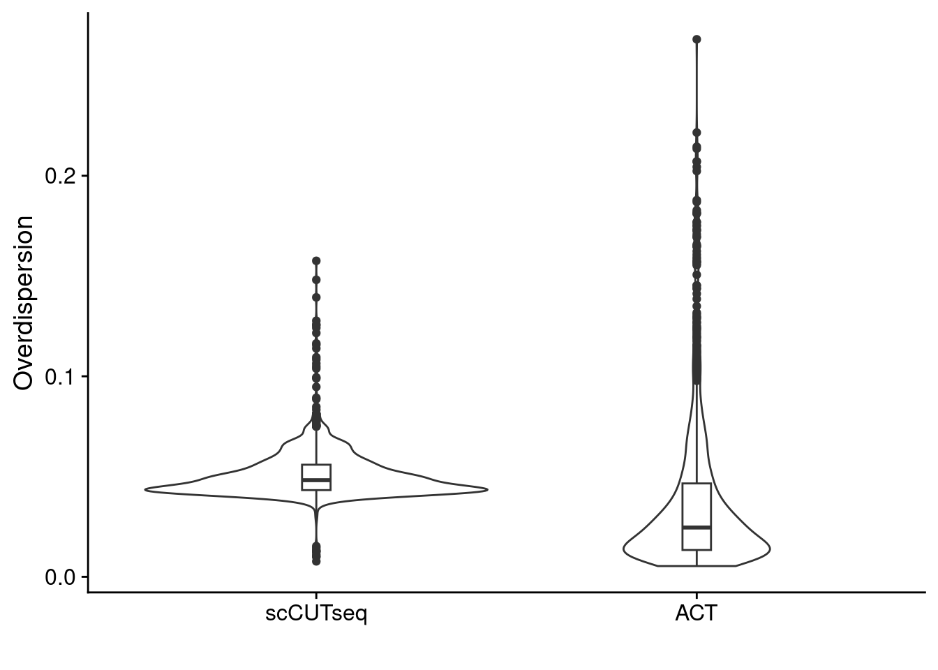
5.3 Plot genomewide heatmaps of ACT and scCUTseq copynumber profiles
Plot both the ACT and scCUTseq genomewide heatmap to visually compare the two methods. Note: the plotting of these can take a while. Furthermore, we set dendrogram = FALSE since there is a known bug with the ggdendro package when you have many samples that are identical (in our case, diploid cells)
# Load in data
p3_sccut = readRDS("./data/P3_cnv.rds")

# Select HQ cells
p3_sccut_profiles = p3_sccut$copynumber[, p3_sccut$stats[classifier_prediction == "good", sample], with = FALSE]
p3_sccut_profiles = p3_sccut_profiles[, grepl("NZ186|MS80|NZ187|NZ188|NZ189|NZ211", colnames(p3_sccut_profiles)), with = F] # Select sections that also has ACT sequencing data

# Make annotation table for scCUTseq
p3_annot = fread("./annotation/P3.tsv", header = FALSE)

scCUT_annot = data.table(sample = colnames(p3_sccut_profiles),
                         variable = "section",
                         value = gsub("_.*", "", colnames(p3_sccut_profiles)))

# Merge to get section information
scCUT_annot = merge(scCUT_annot, p3_annot, by.x = "value", by.y = "V1")

# Plot scCUTseq heatmap
plotHeatmap(p3_sccut_profiles, p3_sccut$bins, dendrogram = FALSE, annotation = scCUT_annot[, .(sample, variable, V2)])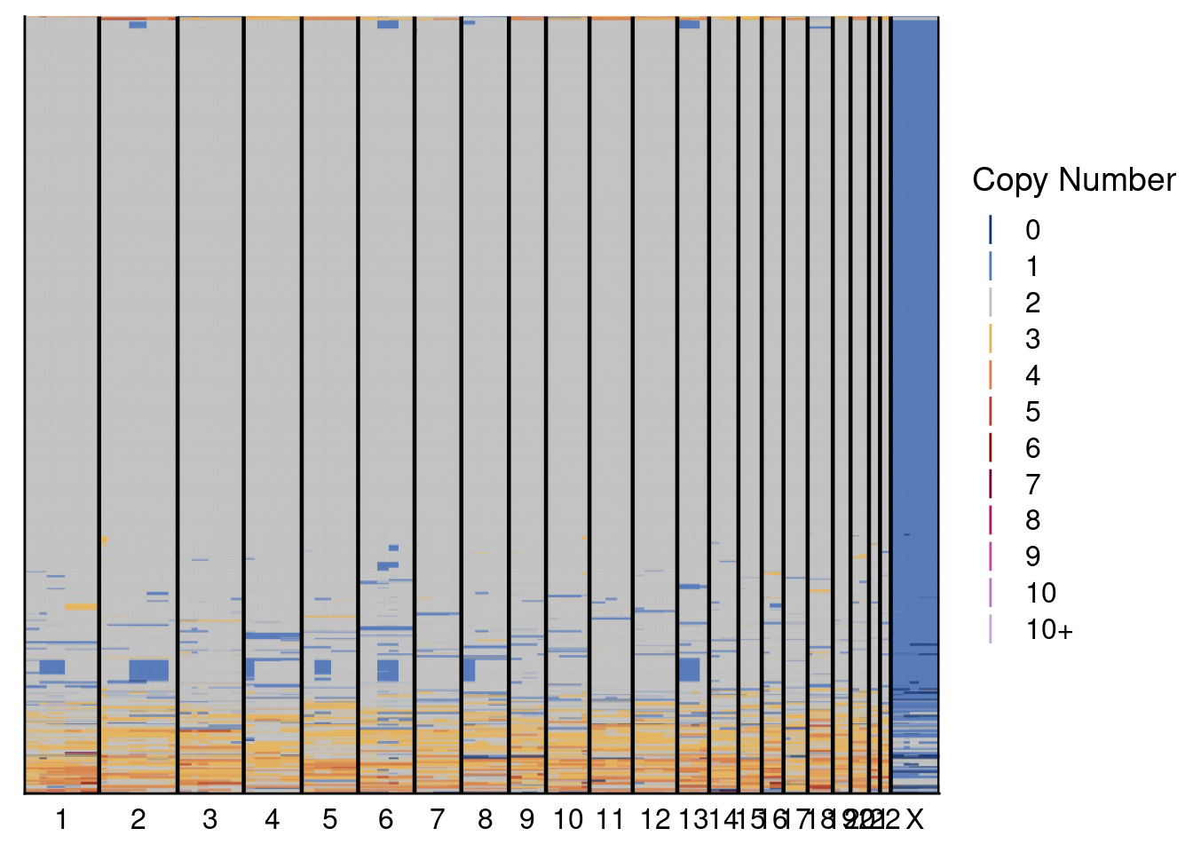
# Get ACT profiles and make annotation
p3_act = readRDS("./data/P3_ACT.rds")
p3_act_profiles = p3_act$copynumber[, sort(p3_act$stats[classifier_prediction == "good", sample]), with = F]

# Make annotation for ACT
ACT_annot = data.table(sample = colnames(p3_act_profiles),
                       variable = "section",
                       value = gsub("_.*", "", colnames(p3_act_profiles)))

# Plot ACT heatmap
plotHeatmap(p3_act_profiles, p3_act$bins, dendrogram = FALSE, annotation = ACT_annot)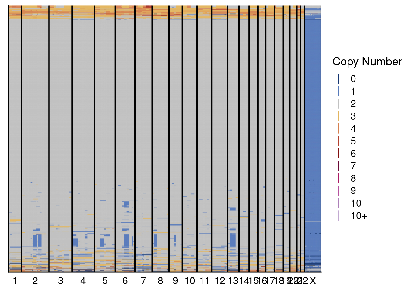
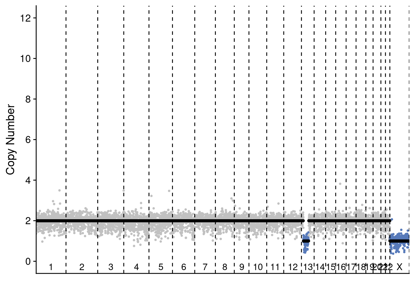
5.4 Plot profile plots of example profiles
We selected 2 profiles of scCUTseq and 2 profiles of ACT to show the differences. These are selected manually but are representative for other plots (you can change the sample ID to manually check others)
# profile selection
sccut = readRDS("./data/CD27.rds")
act = readRDS("./data/CD1p.rds")

# scCUTseq cell 1
plotProfile(sccut$copynumber$AGCCAACGGCA, sccut$counts_gc$AGCCAACGGCA * sccut$ploidies[sample == "AGCCAACGGCA", ploidy], sccut$bins)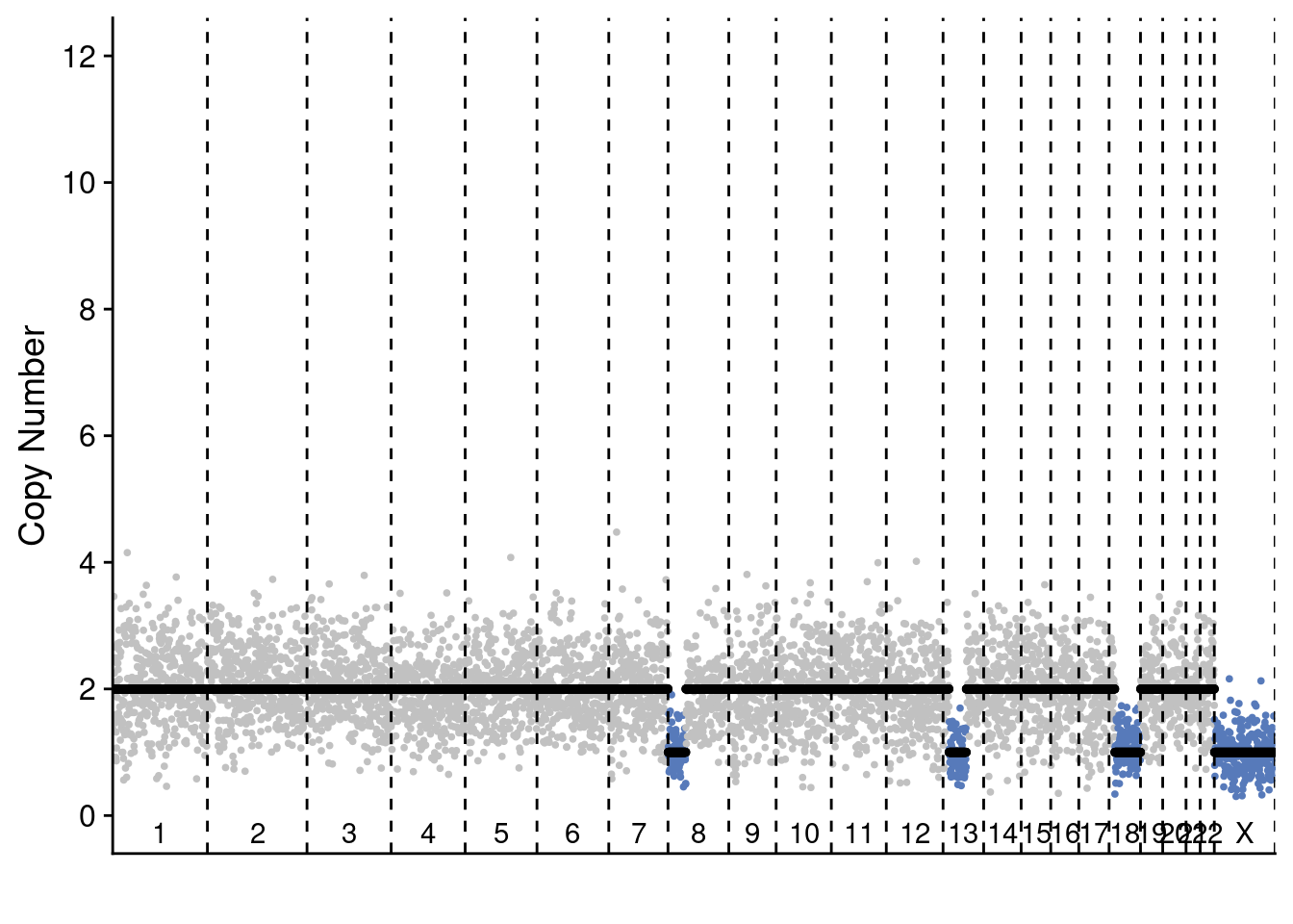
# scCUTseq cell 2
plotProfile(sccut$copynumber$AGCTTGCTCAT, sccut$counts_gc$AGCTTGCTCAT * sccut$ploidies[sample == "AGCTTGCTCAT", ploidy], sccut$bins)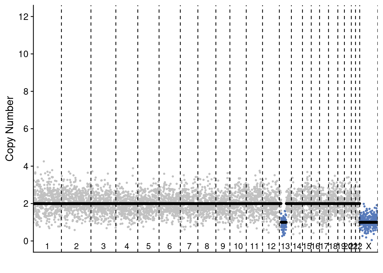
# ACT cell 1
plotProfile(act$copynumber$`296_S296`, act$counts_gc$`296_S296` * act$ploidies[sample == "296_S296", ploidy], act$bins)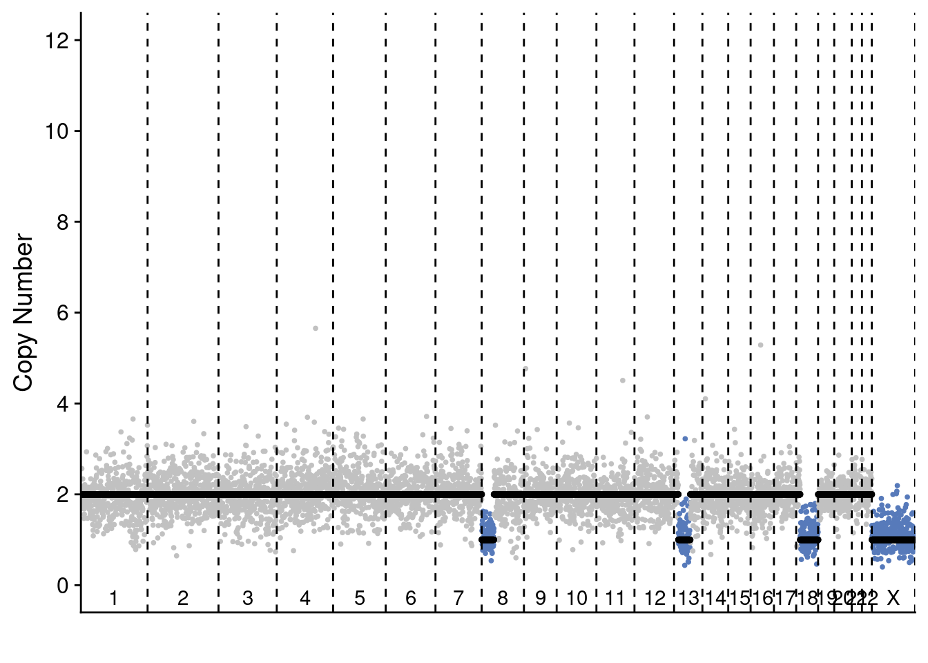
# ACT cell 2
plotProfile(act$copynumber$`227_S227`, act$counts_gc$`227_S227` * act$ploidies[sample == "227_S227", ploidy], act$bins)