6 Spatially resolved single-cell CNA profiling across the prostate
This section produces all the figures used for Figure 1.
6.1 Spatial pathologist annotation
Load in pathologist annotation data
p3_annot = fread("./annotation/P3.tsv", header = FALSE, col.names = c("library", "section", "pathology_annotation"))
p6_annot = fread("./annotation/P6.tsv", header = FALSE, col.names = c("library", "section", "pathology_annotation"))
Plot the annotation data in the schematic of the prostate of both patients.
# Extract x and y coordinates
p3_annot[, x := as.numeric(gsub("L|C.", "", section))]
p3_annot[, y := as.numeric(gsub("L.|C", "", section))]

p6_annot[, x := as.numeric(gsub("L|C.", "", section))]
p6_annot[, y := as.numeric(gsub("L.|C", "", section))]

# Plot
ggplot(p3_annot, aes(x = x, y = y, fill = pathology_annotation)) +
  geom_tile() +
  geom_hline(yintercept = seq(from = .5, to = max(p3_annot$y), by = 1)) +
  geom_vline(xintercept = seq(from = .5, to = max(p3_annot$x), by = 1)) +
  scale_fill_npg() +
  labs(title = "P3 Pathology annotation") +
  scale_y_reverse(expand = c(0, 0), breaks = seq(1, max(p3_annot$y)), labels = seq(1, max(p3_annot$y))) +
  scale_x_reverse(expand = c(0, 0), breaks = seq(1, max(p3_annot$x)), labels = seq(1, max(p3_annot$x))) +
  theme(axis.title = element_blank())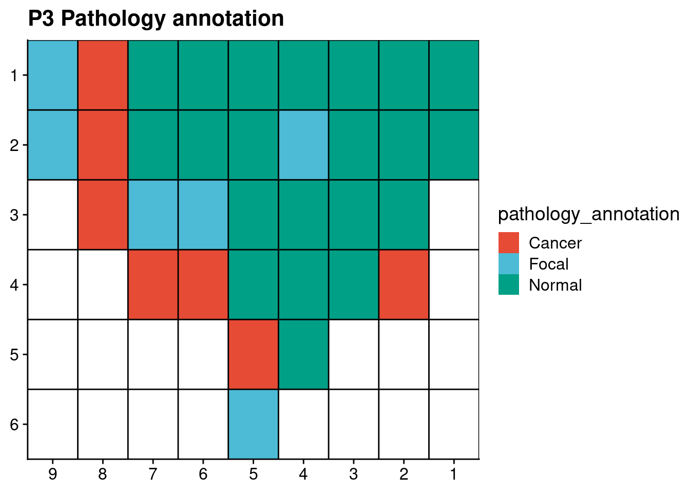
ggplot(p6_annot, aes(x = x, y = y, fill = pathology_annotation)) +
  geom_tile() +
  geom_hline(yintercept = seq(from = .5, to = max(p6_annot$y), by = 1)) +
  geom_vline(xintercept = seq(from = .5, to = max(p6_annot$x), by = 1)) +
  scale_fill_npg() +
  labs(title = "P6 Pathology annotation") +
  scale_y_reverse(expand = c(0, 0), breaks = seq(1, max(p6_annot$y)), labels = seq(1, max(p6_annot$y))) +
  scale_x_reverse(expand = c(0, 0), breaks = seq(1, max(p6_annot$x)), labels = seq(1, max(p6_annot$x))) +
  theme(axis.title = element_blank())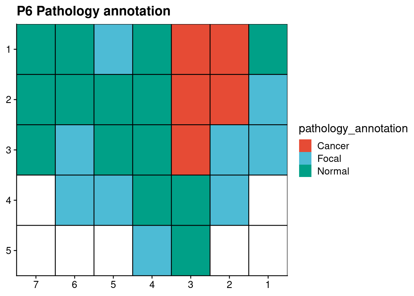
6.2 Spatial distribution of RNAseq clusters, SCNAs and mutations in prostate
Load in RNAseq clusters, copynumber profiles and mutations. In the case of % of cells with SCNAs, we take all the completely diploid cells and take 1 - (fraction of diploid) to get cells with SCNAs.
# Patient 3
p3_cnv = readRDS("data/P3_cnv.rds")
p3_rnaseq = fread("data/P3_RNAseq_clusters.tsv")
p3_mutations = fread("data/P3_nMuts.tsv")

# Patient 6
p6_cnv = readRDS("data/P6_cnv.rds")
p6_rnaseq = fread("data/P6_RNAseq_clusters.tsv")
p6_mutations = fread("data/P6_nMuts.tsv")
Classifiy copynumber profiles into the three cell groups based on the percentage of the genome that is altered and plot the percentages.
profiles = p3_cnv$copynumber[, p3_cnv$stats[classifier_prediction == "good", sample], with = FALSE]
bins = p3_cnv$bins

# Remove all fully diploid cells
diploid_vector = c(rep(2, sum(bins$chr != "X")), rep(1, sum(bins$chr == "X")))

# Keep
diploid_check = sapply(colnames(profiles), function(cell) {
  sum(profiles[[cell]] != diploid_vector)
})

dt = data.table(sample = names(diploid_check), num_altered = diploid_check)

# Divide based on number of alterations
diploid_p3 = profiles[, dt[num_altered == 0, sample], with = FALSE]
pseudodiploid_p3 = profiles[, dt[num_altered != 0 & num_altered <= .25 * nrow(bins), sample], with = FALSE]
monster_p3 = profiles[, dt[num_altered != 0 & num_altered > .25 * nrow(bins), sample], with = FALSE]

# Make into DT for plotting
overall_p3 = data.table(cell_type = c("diploid", "pseudodiploid", "monster"),
                        number = c(ncol(diploid_p3),
                                   ncol(pseudodiploid_p3),
                                   ncol(monster_p3)),
                        patient = "P3")
overall_p3[, percent := number / sum(number) * 100]
profiles = p6_cnv$copynumber[, p6_cnv$stats[classifier_prediction == "good", sample], with = FALSE]
bins = p6_cnv$bins
# Remove all fully diploid cells
diploid_vector = c(rep(2, sum(bins$chr != "X")), rep(1, sum(bins$chr == "X")))
# Keep
diploid_check = sapply(colnames(profiles), function(cell) {
sum(profiles[[cell]] != diploid_vector)
})
dt = data.table(sample = names(diploid_check), num_altered = diploid_check)
# Divide based on number of alterations
diploid_p6 = profiles[, dt[num_altered == 0, sample], with = FALSE]
pseudodiploid_p6 = profiles[, dt[num_altered != 0 & num_altered <= .25 * nrow(bins), sample], with = FALSE]
monster_p6 = profiles[, dt[num_altered != 0 & num_altered > .25 * nrow(bins), sample], with = FALSE]
# Make into DT for plotting
overall_p6 = data.table(cell_type = c("diploid", "pseudodiploid", "monster"),
number = c(ncol(diploid_p6),
ncol(pseudodiploid_p6),
ncol(monster_p6)),
patient = "P6")
overall_p6[, percent := number / sum(number) * 100]Prepare the data for plotting. RNAseq and mutations are ready for plotting (just add coordinates) but we still need to extract the percentage of cells that have SCNAs from the copynumber profiles. We use the previously compiled list of diploid cells for this.
# Make data.table with cell names and type
# P3
dt_p3 = data.table(sample = c(colnames(diploid_p3),
                              colnames(pseudodiploid_p3),
                              colnames(monster_p3)),
                   celltype = c(rep("diploid", ncol(diploid_p3)),
                                rep("pseudodiploid", ncol(pseudodiploid_p3)),
                                rep("monster", ncol(monster_p3))))
dt_p3[, library := gsub("_.*", "", sample)]

# P6
dt_p6 = data.table(sample = c(colnames(diploid_p6),
                              colnames(pseudodiploid_p6),
                              colnames(monster_p6)),
                   celltype = c(rep("diploid", ncol(diploid_p6)),
                                rep("pseudodiploid", ncol(pseudodiploid_p6)),
                                rep("monster", ncol(monster_p6))))
dt_p6[, library := gsub("_.*", "", sample)]

# Get counts per section
total_p3 = dt_p3[, .N, by = .(library)]
total_p6 = dt_p6[, .N, by = .(library)]

# Get diploid counts per section
count_p3 = dt_p3[celltype == "diploid", .N, by = .(library)]
count_p6 = dt_p6[celltype == "diploid", .N, by = .(library)]

# Merge and get fraction of non-diploid (1-diploid)
count_p3 = merge(count_p3, total_p3, by = "library")
count_p6 = merge(count_p6, total_p6, by = "library")

count_p3[, nondiploid_fraction := 1 - (N.x / N.y)]
count_p6[, nondiploid_fraction := 1 - (N.x / N.y)]

# Merge with annotation
count_p3 = merge(count_p3, p3_annot)
count_p6 = merge(count_p6, p6_annot)

# Get coordinates
count_p3[, x := as.numeric(gsub("L|C.", "", section))]
count_p3[, y := as.numeric(gsub("L.|C", "", section))]

count_p6[, x := as.numeric(gsub("L|C.", "", section))]
count_p6[, y := as.numeric(gsub("L.|C", "", section))]
Plot all the data for Patient 3
# Plot RNAseq clusters
p3_rnaseq[, x := as.numeric(gsub("L|C.", "", V1))]
p3_rnaseq[, y := as.numeric(gsub("L.|C", "", V1))]
p3_rnaseq[, V3 := factor(V3, levels = c("2", "1", "3"))]

ggplot(p3_rnaseq, aes(x = x, y = y, fill = V3)) +
  geom_tile() +
  scale_fill_npg() +
  geom_hline(yintercept = seq(from = .5, to = max(p3_rnaseq$y), by = 1)) +
  geom_vline(xintercept = seq(from = .5, to = max(p3_rnaseq$x), by = 1)) +
  labs(title = "RNA-seq clusters (P3)") +
  scale_y_reverse(expand = c(0, 0 ), breaks = seq(1, max(p3_rnaseq$y)), labels = seq(1, max(p3_rnaseq$y))) +
  scale_x_reverse(expand = c(0, 0 ), breaks = seq(1, max(p3_rnaseq$x)), labels = seq(1, max(p3_rnaseq$x))) +
  theme(axis.title = element_blank())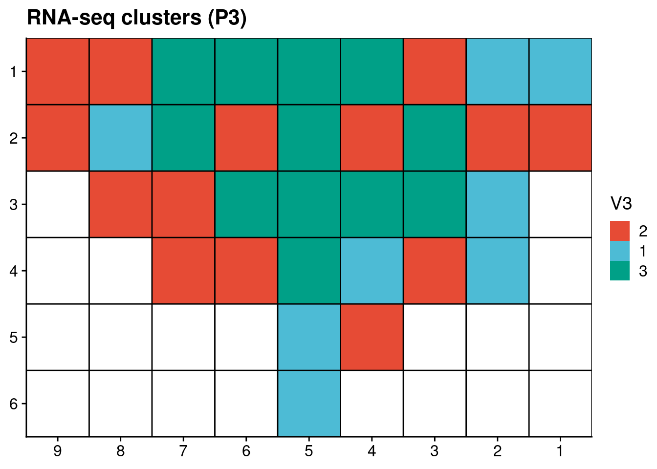
# Plot SCNAs
ggplot(count_p3, aes(x = x, y = y, fill = nondiploid_fraction)) +
  geom_tile() +
  scale_fill_distiller(name = "Percentage of cells\nwith SCNAs", palette = "Reds", direction = 1, na.value = "grey", label = scales::percent_format()) +
  geom_hline(yintercept = seq(from = .5, to = max(count_p3$y), by = 1)) +
  geom_vline(xintercept = seq(from = .5, to = max(count_p3$x), by = 1)) +
  labs(title = "Percentage of cells with SCNAs (P3)") +
  scale_y_reverse(expand = c(0, 0 ), breaks = seq(1, max(count_p3$y)), labels = seq(1, max(count_p3$y))) +
  scale_x_reverse(expand = c(0, 0 ), breaks = seq(1, max(count_p3$x)), labels = seq(1, max(count_p3$x))) +
  theme(axis.title = element_blank())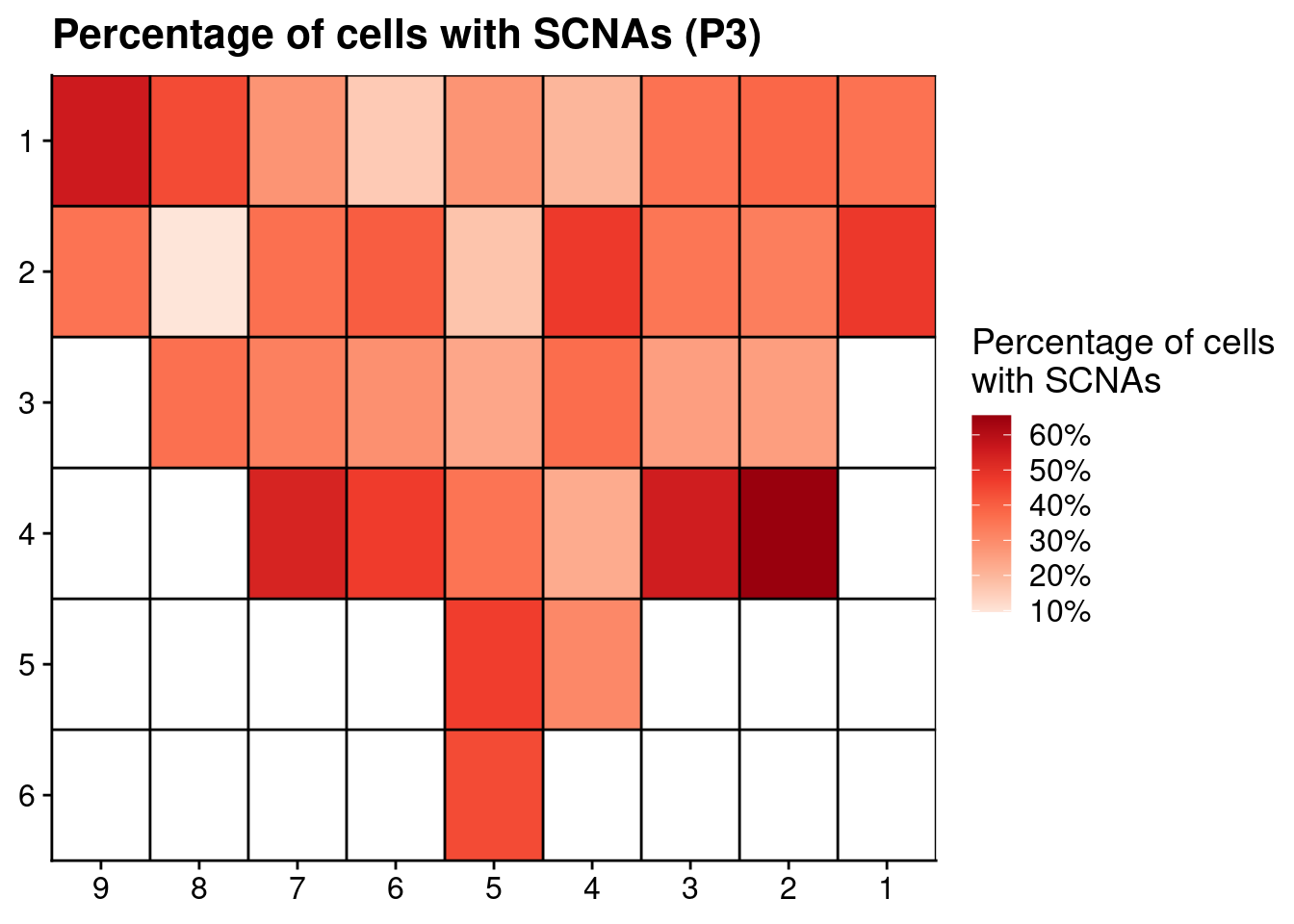
# Plot number of mutations
p3_mutations[, x := as.numeric(gsub("L|C.", "", section))]
p3_mutations[, y := as.numeric(gsub("L.|C", "", section))]

ggplot(p3_mutations, aes(x = x, y = y, fill = n_muts)) +
  geom_tile() +
  scale_fill_distiller(name = "Percentage of cells\nwith SCNAs", palette = "Reds", direction = 1, na.value = "grey", limit = c(0, 12)) +
  geom_hline(yintercept = seq(from = .5, to = max(p3_mutations$y), by = 1)) +
  geom_vline(xintercept = seq(from = .5, to = max(p3_mutations$x), by = 1)) +
  labs(title = "Number of mutations per section (P3)") +
  scale_y_reverse(expand = c(0, 0 ), breaks = seq(1, max(p3_mutations$y)), labels = seq(1, max(p3_mutations$y))) +
  scale_x_reverse(expand = c(0, 0 ), breaks = seq(1, max(p3_mutations$x)), labels = seq(1, max(p3_mutations$x))) +
  theme(axis.title = element_blank())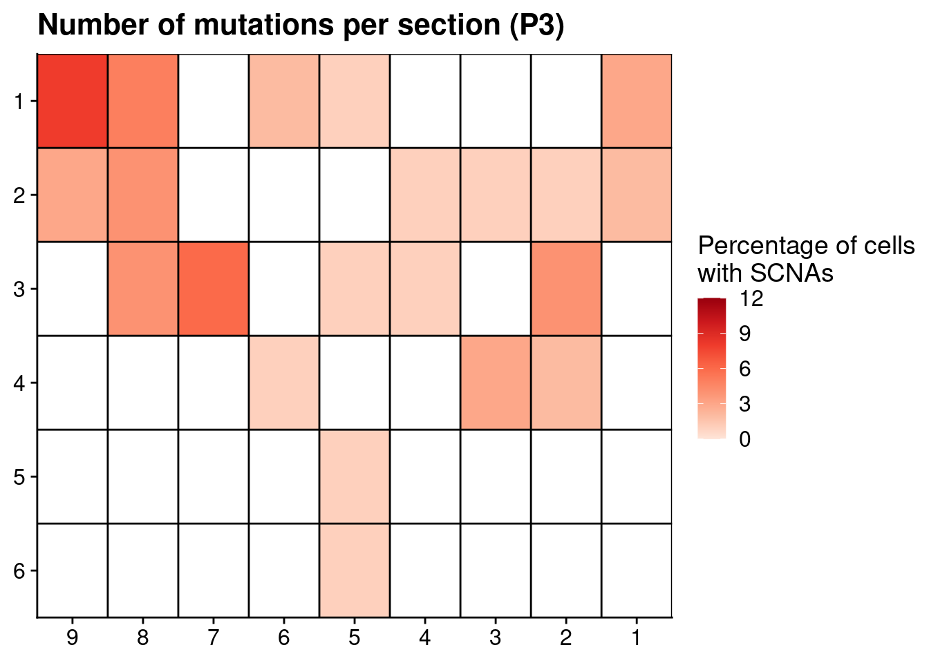
Plot all the data for Patient 6
# Plot RNAseq clusters
p6_rnaseq[, x := as.numeric(gsub("L|C.", "", V1))]
p6_rnaseq[, y := as.numeric(gsub("L.|C", "", V1))]
p6_rnaseq[, V3 := factor(V3, levels = c("2", "1", "3"))]

ggplot(p6_rnaseq, aes(x = x, y = y, fill = V3)) +
  geom_tile() +
  scale_fill_npg() +
  geom_hline(yintercept = seq(from = .5, to = max(p6_rnaseq$y), by = 1)) +
  geom_vline(xintercept = seq(from = .5, to = max(p6_rnaseq$x), by = 1)) +
  labs(title = "RNA-seq clusters (P6)", fill = "RNA-seq cluster") +
  scale_y_reverse(expand = c(0, 0 ), breaks = seq(1, max(p6_rnaseq$y)), labels = seq(1, max(p6_rnaseq$y))) +
  scale_x_reverse(expand = c(0, 0 ), breaks = seq(1, max(p6_rnaseq$x)), labels = seq(1, max(p6_rnaseq$x))) +
  theme(axis.title = element_blank())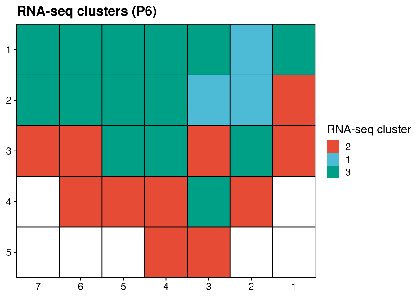
# Plot SCNAs
ggplot(count_p6, aes(x = x, y = y, fill = nondiploid_fraction)) +
  geom_tile() +
  scale_fill_distiller(name = "Percentage of cells\nwith SCNAs", palette = "Reds", direction = 1, na.value = "grey", label = scales::percent_format()) +
  geom_hline(yintercept = seq(from = .5, to = max(count_p6$y), by = 1)) +
  geom_vline(xintercept = seq(from = .5, to = max(count_p6$x), by = 1)) +
  labs(title = "Percentage of cells with SCNAs (P6)") +
  scale_y_reverse(expand = c(0, 0 ), breaks = seq(1, max(count_p6$y)), labels = seq(1, max(count_p6$y))) +
  scale_x_reverse(expand = c(0, 0 ), breaks = seq(1, max(count_p6$x)), labels = seq(1, max(count_p6$x))) +
  theme(axis.title = element_blank())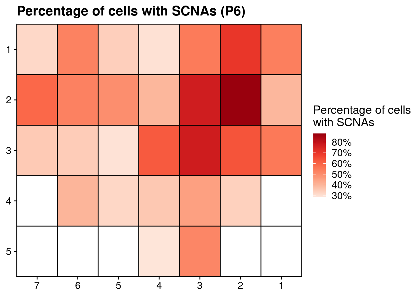
# Plot number of mutations
p6_mutations[, x := as.numeric(gsub("L|C.", "", section))]
p6_mutations[, y := as.numeric(gsub("L.|C", "", section))]

ggplot(p6_mutations, aes(x = x, y = y, fill = n_muts)) +
  geom_tile() +
  scale_fill_distiller(name = "Number of mutations", palette = "Reds", direction = 1, na.value = "grey", limit = c(0, 12)) +
  geom_hline(yintercept = seq(from = .5, to = max(p6_mutations$y), by = 1)) +
  geom_vline(xintercept = seq(from = .5, to = max(p6_mutations$x), by = 1)) +
  labs(title = "Number of mutations per section (P6)") +
  scale_y_reverse(expand = c(0, 0 ), breaks = seq(1, max(p6_mutations$y)), labels = seq(1, max(p6_mutations$y))) +
  scale_x_reverse(expand = c(0, 0 ), breaks = seq(1, max(p6_mutations$x)), labels = seq(1, max(p6_mutations$x))) +
  theme(axis.title = element_blank())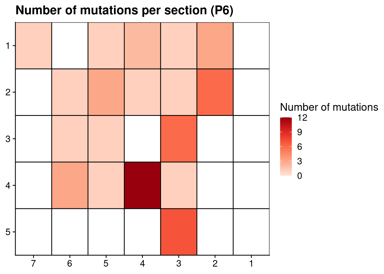
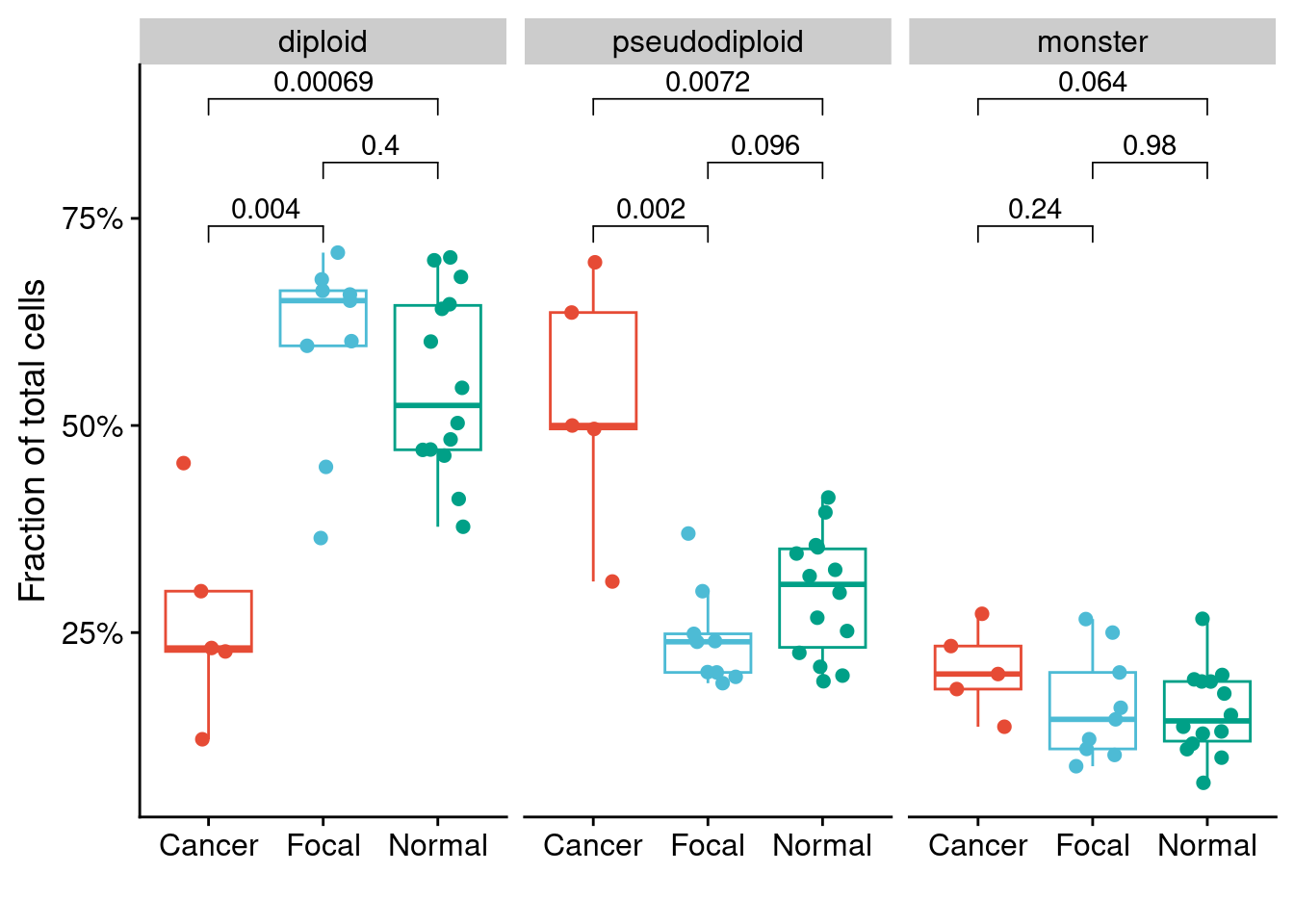
6.3 Cell type distribution
We detected three different major groups of cells, namely, Diploid cells, pseudo-diploid cells, and monster cells. Above, we already assigned our cells to the different celltype so we can now use this to plot the percentages.
# Combine patients
overall = rbind(overall_p3, overall_p6)

# Reorder factors
overall[, cell_type := factor(cell_type, levels = c("diploid", "pseudodiploid", "monster"))]

# Plot
ggplot(overall, aes(x = patient, y = percent, fill = cell_type, label = number)) +
  geom_col() +
  scale_y_continuous(expand = c(0, 0)) +
  labs(y = "Percentage of cell type", x = "", fill = "Cell type") +
  geom_text(aes(label = paste0(round(percent, 1), "%\n(n = ", number, ")")),
                   position = position_stack(vjust = .5), size = 4) +
  scale_fill_npg() +
  theme(axis.ticks.x = element_blank())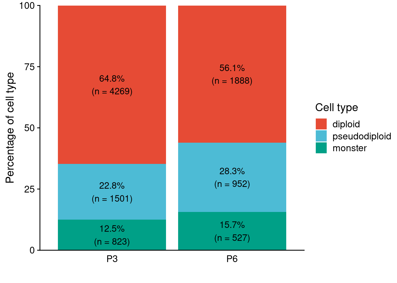
Second, we show representative single-cell profiles for these celltypes.
# Load in plotProfile function to plot copy number profiles
source("functions/plotProfile.R")

# Select random diploid, pseudo-diploid and monster cell for each patient
diploid_p3_example = colnames(diploid_p3)[sample(1:ncol(diploid_p3), 1)]
pseudodiploid_p3_example = colnames(pseudodiploid_p3)[sample(1:ncol(pseudodiploid_p3), 1)]
monster_p3_example = colnames(monster_p3)[sample(1:ncol(monster_p3), 1)]

diploid_p6_example = colnames(diploid_p6)[sample(1:ncol(diploid_p6), 1)]
pseudodiploid_p6_example = colnames(pseudodiploid_p6)[sample(1:ncol(pseudodiploid_p6), 1)]
monster_p6_example = colnames(monster_p6)[sample(1:ncol(monster_p6), 1)]

# Plot representative profiles for diploid, pseudo-diploid and monster cells
# P3
plotProfile(p3_cnv$copynumber[[diploid_p3_example]], p3_cnv$counts_gc[[diploid_p3_example]] * p3_cnv$ploidies[sample == diploid_p3_example, ploidy], bins = p3_cnv$bins)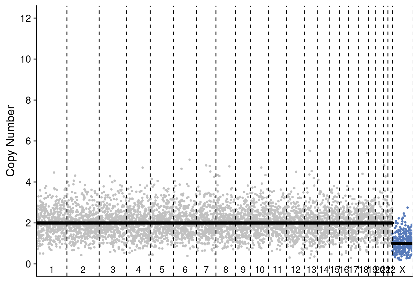
plotProfile(p3_cnv$copynumber[[pseudodiploid_p3_example]], p3_cnv$counts_gc[[pseudodiploid_p3_example]] * p3_cnv$ploidies[sample == pseudodiploid_p3_example, ploidy], bins = p3_cnv$bins)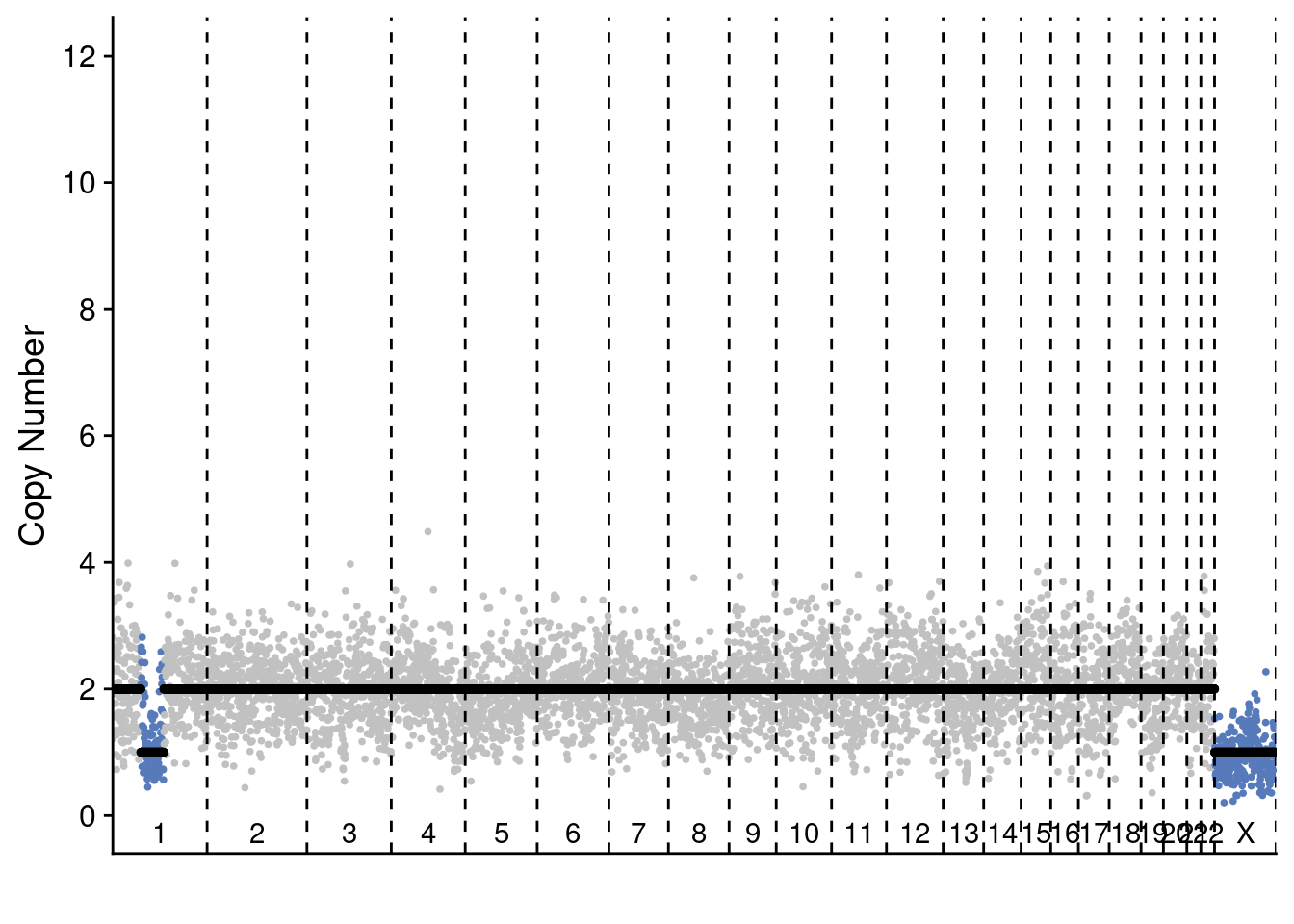
plotProfile(p3_cnv$copynumber[[monster_p3_example]], p3_cnv$counts_gc[[monster_p3_example]] * p3_cnv$ploidies[sample == monster_p3_example, ploidy], bins = p3_cnv$bins)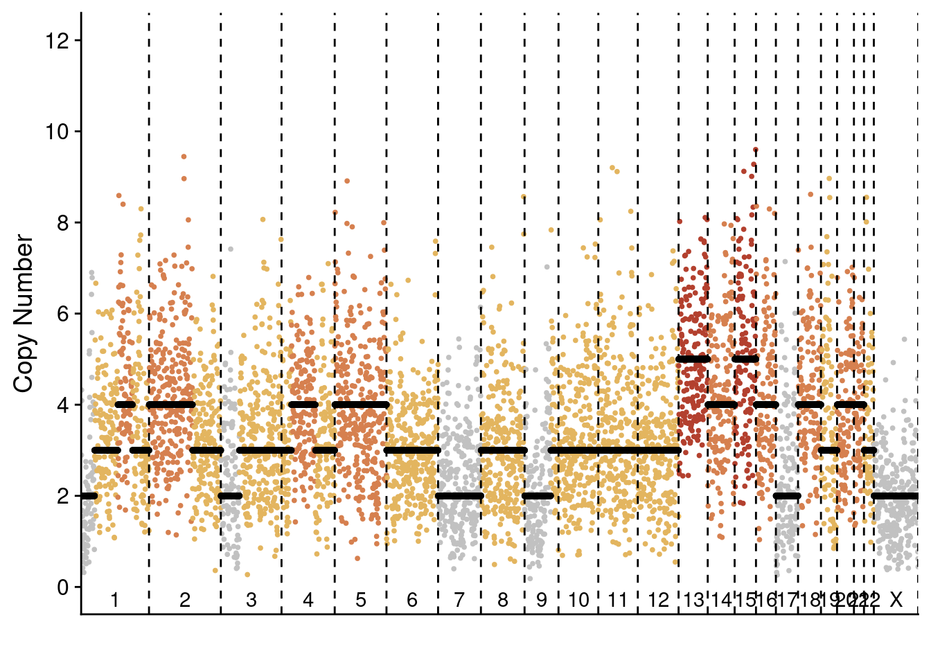
# P6
plotProfile(p6_cnv$copynumber[[diploid_p6_example]], p6_cnv$counts_gc[[diploid_p6_example]] * p6_cnv$ploidies[sample == diploid_p6_example, ploidy], bins = p6_cnv$bins)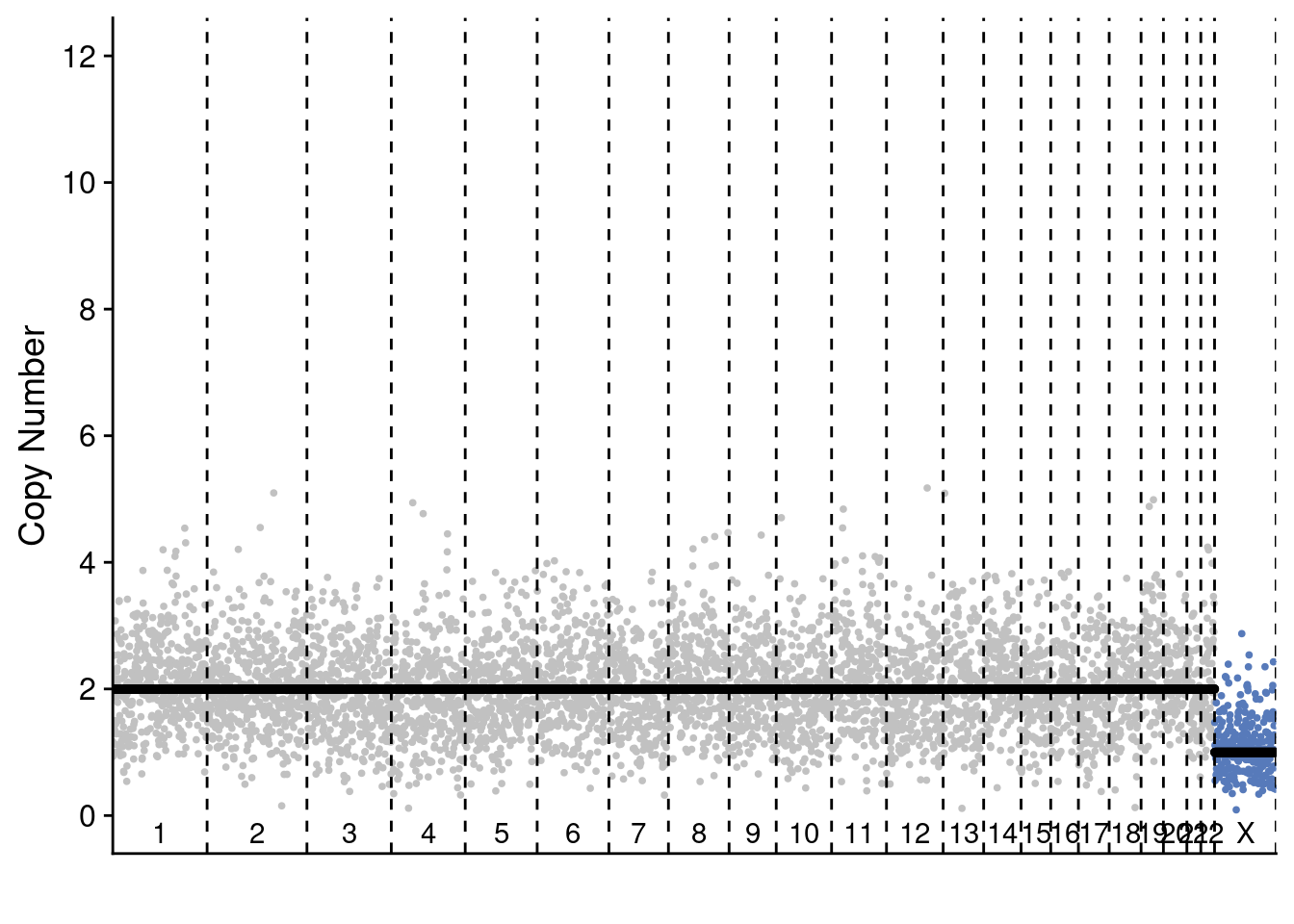
plotProfile(p6_cnv$copynumber[[pseudodiploid_p6_example]], p6_cnv$counts_gc[[pseudodiploid_p6_example]] * p6_cnv$ploidies[sample == pseudodiploid_p6_example, ploidy], bins = p6_cnv$bins)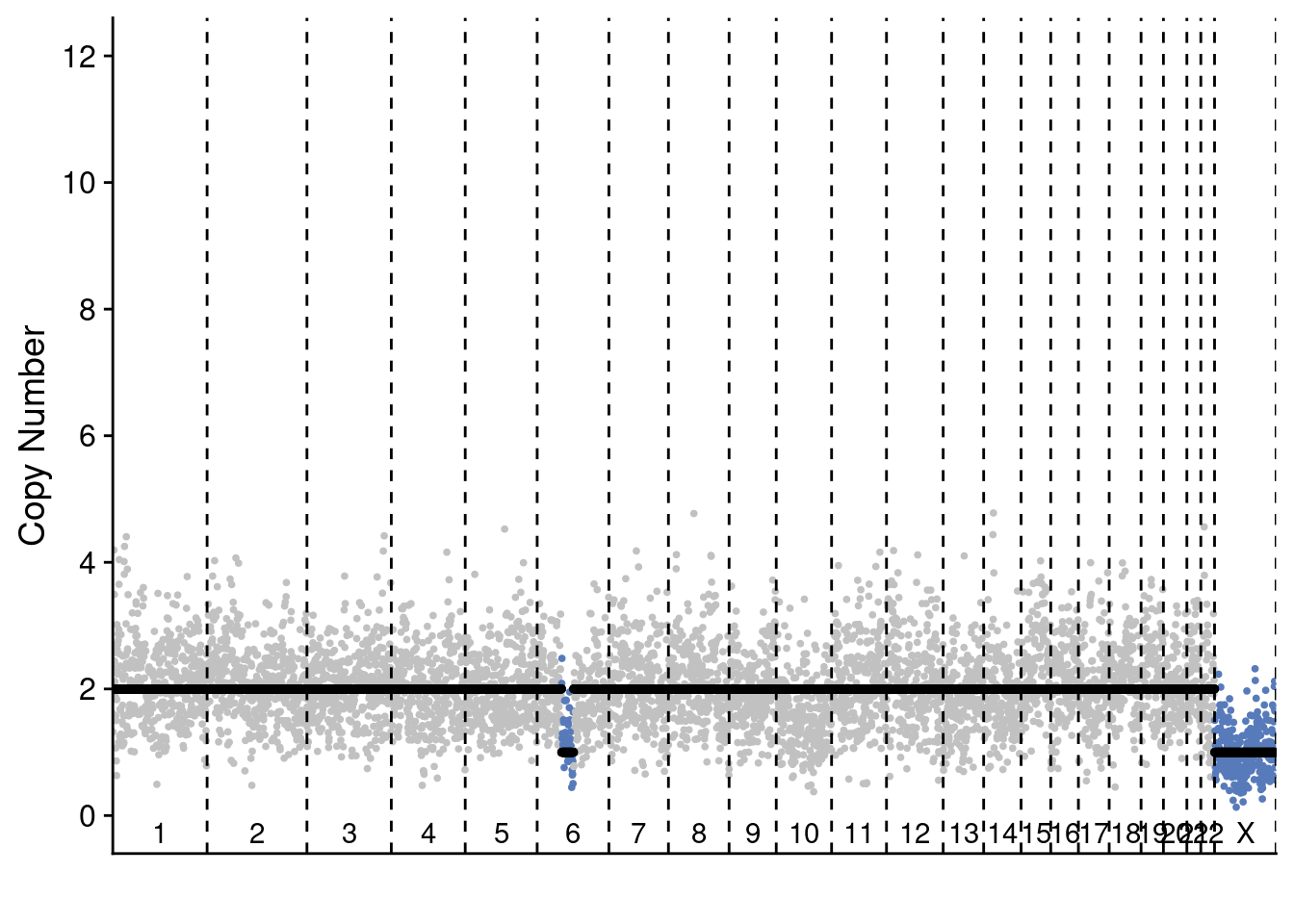
plotProfile(p6_cnv$copynumber[[monster_p6_example]], p6_cnv$counts_gc[[monster_p6_example]] * p6_cnv$ploidies[sample == monster_p6_example, ploidy], bins = p6_cnv$bins)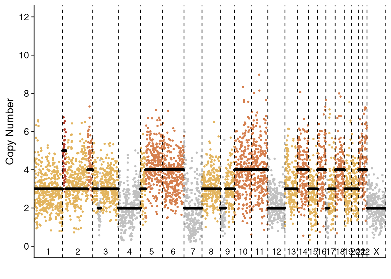 Plot distribution of celltypes in the different regions
# Get counts
counts_p3 = dt_p3[, .N, by = .(celltype, library)]
counts_p6 = dt_p6[, .N, by = .(celltype, library)]

# Merge with annotation
counts_p3 = merge(counts_p3, p3_annot)
counts_p6 = merge(counts_p6, p6_annot)

# Merge with total counts per section (calculated in previous section)
counts_p3 = merge(counts_p3, total_p3)
counts_p6 = merge(counts_p6, total_p6)

# Calculate fraction
counts_p3[, fraction := N.x / N.y]
counts_p6[, fraction := N.x / N.y]

# Reorder factors
counts_p3[, celltype := factor(celltype, levels = c("diploid", "pseudodiploid", "monster"))]
counts_p6[, celltype := factor(celltype, levels = c("diploid", "pseudodiploid", "monster"))]

# Plot P3
ggplot(counts_p3, aes(x = pathology_annotation, y = fraction, color = pathology_annotation)) +
  facet_wrap(~celltype) +
  geom_boxplot(outlier.shape = NA) +
  geom_jitter(width = .25, size = 2) +
  scale_color_npg() +
  scale_y_continuous(labels = scales::percent_format(), breaks = seq(0, 1, .25)) +
  labs(y = "Fraction of total cells", x = "") +
  stat_compare_means(comparisons = list(c("Cancer", "Focal"),
                                        c("Focal", "Normal"),
                                        c("Cancer", "Normal"))) +
  theme(legend.position = "")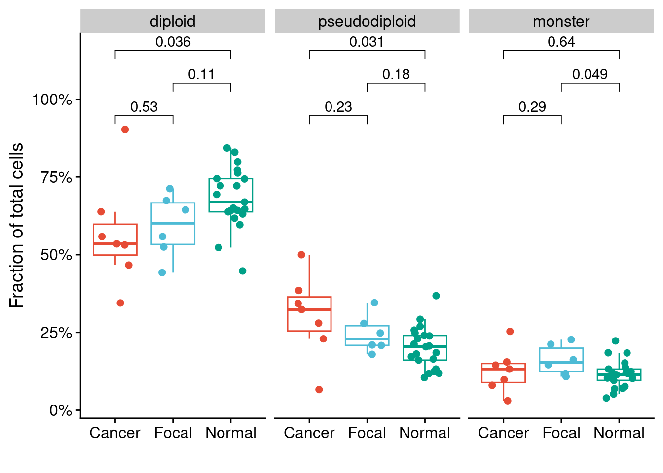
# Plot P6
ggplot(counts_p6, aes(x = pathology_annotation, y = fraction, color = pathology_annotation)) +
  facet_wrap(~celltype) +
  geom_boxplot(outlier.shape = NA) +
  geom_jitter(width = .25, size = 2) +
  scale_color_npg() +
  scale_y_continuous(labels = scales::percent_format(), breaks = seq(0, 1, .25)) +
  labs(y = "Fraction of total cells", x = "") +
  stat_compare_means(comparisons = list(c("Cancer", "Focal"),
                                        c("Focal", "Normal"),
                                        c("Cancer", "Normal"))) +
  theme(legend.position = "")